Outline. This section shows that second order derivatives of the output function vanish during flat minimum search. This justifies the linear approximations in section 4.
Intuition.
We show that the algorithm tends to suppress the following values:
(1) unit activations,
(2) first order activation derivatives,
(3) the sum of all contributions
of an arbitrary unit activation to the net
output.
Since weights, inputs, activation functions,
and their first and second
order derivatives are bounded,
the entries in the
Hessian decrease
where the corresponding
![]() increase.
increase.
Formal details.
We consider a strictly layered
feedforward network with ![]() output units and
output units and
![]() layers.
We use the same activation function
layers.
We use the same activation function ![]() for all units.
For simplicity, in what follows we focus on a single
input vector
for all units.
For simplicity, in what follows we focus on a single
input vector ![]() .
.
![]() (and occasionally
(and occasionally ![]() itself) will be notationally suppressed.
We have
itself) will be notationally suppressed.
We have
The last term of equation (1) (the ``regulator'') expresses output sensitivity (to be minimized) with respect to simultaneous perturbations of all weights. ``Regulation'' is done by equalizing the sensitivity of the output units with respect to the weights. The ``regulator'' does not influence the same particular units or weights for each training example. It may be ignored for the purposes of this section. Of course, the same holds for the first (constant) term in (1). We are left with the second term. With (34) we obtain:
Let us have a closer look at this equation. We observe:
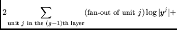
(1) Activations of units decrease in proportion
to their fan-outs.
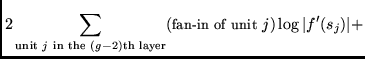
(2) First order derivatives of the activation functions
decrease in proportion to their fan-ins.
(3) A term of the form
![]() expresses the sum of
unit
expresses the sum of
unit ![]() 's
squared contributions
to the net output.
Here
's
squared contributions
to the net output.
Here ![]() ranges over
ranges over
![]() ,
and unit
,
and unit ![]() is in the
is in the ![]() th layer
(for the special case
th layer
(for the special case ![]() ,
we get
,
we get
![]() ).
These terms also decrease
in proportion to unit
).
These terms also decrease
in proportion to unit ![]() 's fan-in.
Analogously,
equation (35) can be extended to the case of additional layers.
's fan-in.
Analogously,
equation (35) can be extended to the case of additional layers.
Comment.
Let us assume
that ![]() and
and ![]() is ``difficult to achieve''
(can be achieved only by fine-tuning all weights on
connections to unit
is ``difficult to achieve''
(can be achieved only by fine-tuning all weights on
connections to unit ![]() ).
Instead of minimizing
).
Instead of minimizing
![]() or
or ![]() by adjusting the net input of unit
by adjusting the net input of unit ![]() (this requires fine-tuning of many weights),
our algorithm prefers
pushing weights
(this requires fine-tuning of many weights),
our algorithm prefers
pushing weights ![]() on connections to output units
towards zero (other weights are less affected).
On the other hand,
if
on connections to output units
towards zero (other weights are less affected).
On the other hand,
if ![]() and
and ![]() is not ``difficult to achieve'',
then, unlike weight decay, our algorithm
does not necessarily prefer
weights close to zero.
Instead, it prefers (possibly very strong)
weights which push
is not ``difficult to achieve'',
then, unlike weight decay, our algorithm
does not necessarily prefer
weights close to zero.
Instead, it prefers (possibly very strong)
weights which push ![]() or
or ![]() towards zero
(e.g., with sigmoid units active in [0,1]:
strong inhibitory weights are preferred; with Gaussian units:
high absolute weight values are preferred).
See the experiment in section 5.2.
towards zero
(e.g., with sigmoid units active in [0,1]:
strong inhibitory weights are preferred; with Gaussian units:
high absolute weight values are preferred).
See the experiment in section 5.2.
How does this influence the Hessian?
The entries in the Hessian corresponding to
output ![]() can be written as follows:
can be written as follows:
According to the analysis above,
the first order derivatives in the second term of (36)
are pushed towards zero. So are the
![]() of the sum in the second term of (36).
of the sum in the second term of (36).
The only remaining expressions of interest are second order derivatives of
units in layer ![]() .
The
.
The
![]() are bounded if
(a) the weights, (b) the activation functions, (c)
their first and second order
derivatives, and (d) the inputs are bounded.
This is indeed the case, as will be shown for
networks with one or two hidden layers:
are bounded if
(a) the weights, (b) the activation functions, (c)
their first and second order
derivatives, and (d) the inputs are bounded.
This is indeed the case, as will be shown for
networks with one or two hidden layers:
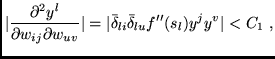
Case 1: For unit ![]() in a single hidden layer (
in a single hidden layer (![]() ),
we obtain
),
we obtain
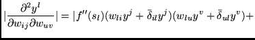
Case 2: For unit ![]() in the third layer
of a net with 2 hidden layers (
in the third layer
of a net with 2 hidden layers (![]() ),
we obtain
),
we obtain
Conclusion:
As desired,
our algorithm makes the
![]() decrease where
decrease where
![]() or
or
![]() increase.
increase.