


Next: DERIVATION OF THE ALGORITHM
Up: FLAT MINIMA NEURAL COMPUTATION
Previous: TASK / ARCHITECTURE /
THE ALGORITHM
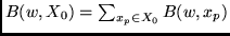
Let
 denote the inputs of the training set.
We approximate
denote the inputs of the training set.
We approximate  by
by  , where
is defined like in the previous
section (replacing
, where
is defined like in the previous
section (replacing  by
by  ).
For simplicity, in what follows, we will abbreviate
by
).
For simplicity, in what follows, we will abbreviate
by  .
Starting with a random initial weight vector,
flat minimum search (FMS)
tries to find a
.
Starting with a random initial weight vector,
flat minimum search (FMS)
tries to find a  that not only has low
  but also defines a box
  with maximal
box volume
with maximal
box volume  and, consequently, minimal
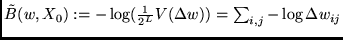 .
Note the relationship to MDL:
.
Note the relationship to MDL:  is the number of bits required
to describe the weights, whereas
the number of bits needed to describe the
is the number of bits required
to describe the weights, whereas
the number of bits needed to describe the  ,
given
(with
,
given
(with
 ),
can be bounded by fixing
),
can be bounded by fixing  (see appendix A.1).
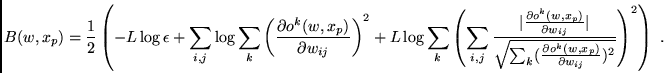
In the next section we derive the following algorithm.
We use gradient descent to minimize
(see appendix A.1).
In the next section we derive the following algorithm.
We use gradient descent to minimize
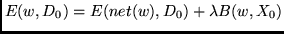 ,
where
,
where
 , and
, and
 |
(1) |
Here  is the activation of the
  th output unit
(given weight vector and input
th output unit
(given weight vector and input  ),
),
 is a constant, and
 is
the regularization constant (or hyperparameter) which controls
the trade-off between regularization and training error (see appendix A.1).
To minimize
is
the regularization constant (or hyperparameter) which controls
the trade-off between regularization and training error (see appendix A.1).
To minimize  ,
for each
,
for each  we have to compute
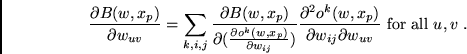 |
(2) |
It can be shown that by
using Pearlmutter's and M ller's
efficient second order method,
the gradient of
ller's
efficient second order method,
the gradient of  can be computed in
  time (see details in A.3).
Therefore, our algorithm
has the same order of computational complexity as standard backprop.
time (see details in A.3).
Therefore, our algorithm
has the same order of computational complexity as standard backprop.
Next: DERIVATION OF THE ALGORITHM
Up: FLAT MINIMA NEURAL COMPUTATION
Previous: TASK / ARCHITECTURE /
Juergen Schmidhuber
2003-02-13
Back to Financial Forecasting page