Experiment 3: Function Approximation / Inductive Transfer

This experimental case study will demonstrate that IS can successfully learn in a changing environment where the tasks to be solved become more and more difficult over time (inductive transfer).

Task sequence. Our system is exposed to a sequence of more and more complex function approximation problems. The functions to be learned are $f_1(x,y) = x + y$; $f_2(x,y,z) = x + y - z$; $f_3(x,y,z) = (x + y - z)^2$; $f_4(x,y,z) = (x + y - z)^4$; $f_5(x,y,z) = (x + y - z)^8$.

Trials. The system's single life is decomposable into $n$ successive trials $A_1$, $A_2$, ..., $A_n$ (but the learner has no a priori concept of a trial). The $i$-th trial lasts from discrete time step $t_i+1$ until discrete time step $t_{i+1}$, where $t_1 = 0$ (system birth) and $t_{n+1} = T$ (system death). In a given trial $A_i$ we first select a function $g_i \in \{f_1, \ldots, f_5 \}$. As the trial number increases, so does the probability of selecting a more complex function. In early trials the focus is on $f_1$. In late trials the focus is on $f_5$. In between there is a gradual shift in task difficulty: using a function pointer $ptr$ (initially 1) and an integer counter $c$ (initially 100), in trial $A_i$ we select $g_i := f_{ptr}$ with probability $\frac{c}{100}$, and $g_i := f_{ptr+1}$ with probability $1-\frac{c}{100}$. If the reward acceleration during the most recent two trials exceeds a certain threshold (0.05), then $c$ is decreased by 1. If $c$ becomes 0 then $f_{ptr}$ is increased by 1, and $c$ is reset to 100. This is repeated until $f_{ptr} := f_5$. From then on, $f_5$ is always selected.

Once $g_i$ is selected, randomly generated real values $x$, $y$ and $z$ are put into work cells 0, 1, 2, respectively. The contents of an arbitrarily chosen work cell (we always use cell 6) are interpreted as the system's response. If $c_6$ fulfills the condition $\vert g_i(x, y, z) - c_6 \vert< 0.0001$, then the trial ends and the current reward becomes $1.0$; otherwise the current reward is 0.0.

Instructions. Instruction sequences can be composed from the following primitive instructions (compare section 4.1):
Add($w_1,w_2,w_3$), Sub($w_1,w_2,w_3$), Mul($w_1,w_2,w_3$), Mov($w_1, w_2$), IncProb($w_1,w_2,w_3$), EndSelfMod($w_1$), JumpHome(). Each instruction occupies 4 successive program cells (some of them unused if the instruction has less than 3 parameters). We use $m = 50, n = 7$.

Evaluation Condition. SSA is called after each 5th consecutive non-zero reward signal after the end of each SMS, i.e., we set $n_{NZR}=5$.

Huge search space. Given the primitives above, random search would require about $10^{17}$ trials on average to find a solution for $f_5$ -- the search space is huge. The gradual shift in task complexity, however, helps IS to learn $f_5$ much faster, as will be seen below.

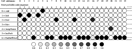
Results. After about $9.4\times 10^{8}$ instruction cycles (ca. $10^8$ trials), the system is able to compute $f_5$ almost perfectly, given arbitrary real-valued inputs. The corresponding speed-up factor over (infeasible) random or exhaustive search is about $10^9$ -- compare paragraph ``Huge search space'' above. The solution (see Figure 5) involves 21 strongly modified probability distributions of the policy (after learning, the correct instructions had extreme probability values). At the end, the most probable code is given by the following integer sequence:

1 2 1 6 1 0 6 6 2 6 6 6 2 6 6 6 2 6 6 6 4 $*$ $*$ $*$...

The corresponding ``program'' and the (very high) probabilities of its instructions and parameters are shown in Table 4.

Figure: The final state of the probability matrix for the function learning problem. Grey scales indicate the magnitude of probabilities of instructions and parameters. The matrix was computed by self-modification sequences generated according to the matrix itself (initially, all probability distributions were maximum entropy distributions).

Table: The final, most probable ``program'' and the corresponding probabilities.

	Probabilities	Instruction	Parameters	Semantics
1.	(0.994, 0.975, 0.991, 0.994)	Sub	( 2, 1, 6)	$(z-y)$ $\Longrightarrow c_6$
2.	(0.994, 0.981, 0.994, 0.994)	Sub	( 0, 6, 6)	$(x-(z-y))$ $\Longrightarrow c_6$
3.	(0.994, 0.994, 0.994, 0.994)	Mul	( 6, 6, 6)	$(x+y-z)^{2}$ $\Longrightarrow c_6$
4.	(0.994, 0.994, 0.994, 0.994)	Mul	( 6, 6, 6)	$(x+y-z)^{4}$ $\Longrightarrow c_6$
5.	(0.869, 0.976, 0.994, 0.994)	Mul	( 6, 6, 6)	$(x+y-z)^{8}$ $\Longrightarrow c_6$
6.	(0.848, --, --, -- )	JumpHome	(-, -, -,)	0 $\Longrightarrow$ IP

Evolution of self-modification frequencies. During its life the system generates a lot of self-modifications to compute the strongly modified policy. This includes changes of the probabilities of self-modifications. It is quite interesting (and also quite difficult) to find out to which extent the system uses self-modifying instructions to learn how to use self-modifying instructions. Figure 6 gives a vague idea of what is going on by showing a typical plot of the frequency of IncProb instructions during system life (sampled at intervals of $10^6$ basic cycles). Soon after its birth, the system found it useful to dramatically increase the frequency of IncProb; near its death (when there was nothing more to learn) it significantly reduced this frequency. This is reminiscent of Schwefel's work (1974) on self-adjusting mutation rates. One major novelty is the adaptive, highly non-uniform distribution of self-modifications on ``promising'' individual policy components.

Figure: Numbers of executed self-modifying instructions plotted against time, sampled at intervals of $10^6$ instruction cycles. The graph reflects that the system soon uses self-modifying instructions to increase the frequency of self-modifying instructions. Near system death the system learns that there is not much to learn any more, and decreases this frequency.

Stack evolution. The temporary ups and downs of the stack reflect that as the tasks change, the system selectively keeps still useful old modifications (corresponding to information conveyed by previous tasks that is still valuable for solving the current task), but deletes modifications that are too much tailored to previous tasks. In the end, there are only about 200 stack entries corresponding to only 200 valid probability modifications - this is a small number compared to the about $5 * 10^5$ self-modifications executed during system life.

Back to Optimal Universal Search page
Back to Reinforcement Learning page
Back to Program Evolution page