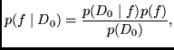
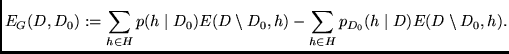
Short Guide Through Appendix A.1. We introduce a novel kind of generalization error that can be split into an overfitting error and an underfitting error. To find hypotheses causing low generalization error, we first select a subset of hypotheses causing low underfitting error. We are interested in those of its elements causing low overfitting error.
More Detailed Guide Through Appendix A.1.
Definitions.
Let
![]() be the set of
all possible input/output pairs (pairs of vectors).
Let
be the set of
all possible input/output pairs (pairs of vectors).
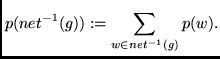
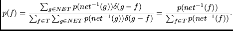
Let ![]() be the set of functions that can be implemented by the network.
For every net function
be the set of functions that can be implemented by the network.
For every net function ![]() we have
we have ![]() .
Elements of
.
Elements of ![]() are parameterized with
a parameter vector
are parameterized with
a parameter vector ![]() from the set of possible parameters
from the set of possible parameters ![]() .
.
![]() is a function which maps a parameter vector
is a function which maps a parameter vector ![]() onto a net function
onto a net function ![]() (
(![]() is surjective.)
Let
is surjective.)
Let ![]() be the set of target functions
be the set of target functions ![]() , where
, where ![]() .
Let
.
Let ![]() be the set of hypothesis functions
be the set of hypothesis functions ![]() , where
, where ![]() .
For simplicity, take all sets to be finite, and let all functions map
each
.
For simplicity, take all sets to be finite, and let all functions map
each ![]() to some
to some ![]() .
Values of functions with argument
.
Values of functions with argument ![]() are
denoted by
are
denoted by
![]() . We have
. We have
![]() .
.
Let
![]() be the data,
where
be the data,
where ![]() .
.
![]() is divided into a training set
is divided into a training set
![]() and a test set
and a test set
![]() .
For the moment,
we are not interested in how
.
For the moment,
we are not interested in how ![]() was obtained.
was obtained.
We use squared error
![]() , where
, where
![]() is the Euclidean norm.
is the Euclidean norm.
![]() .
.
![]() .
.
![]() holds.
holds.
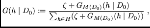
Learning.
We use a variant of the Gibbs formalism (see
Opper & Haussler, 1991,
or Levin et al., 1990).
Consider a stochastic learning algorithm (random weight
initialization, random learning rate).
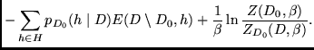
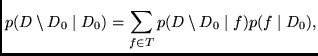
The learning algorithm attempts to reduce training set error by
randomly selecting a hypothesis with low ![]() ,
according to some conditional
distribution
,
according to some conditional
distribution ![]() over
over ![]() .
.
![]() is chosen in advance,
but in contrast to
traditional Gibbs (which deals with unconditional distributions on
is chosen in advance,
but in contrast to
traditional Gibbs (which deals with unconditional distributions on ![]() ),
we may take a look at the training set before selecting
),
we may take a look at the training set before selecting ![]() .
For instance, one training
set may suggest linear functions as being more probable
than others, another one splines, etc.
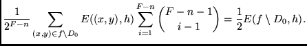
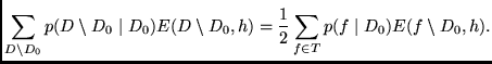
The unconventional Gibbs variant is appropriate because
FMS uses only
.
For instance, one training
set may suggest linear functions as being more probable
than others, another one splines, etc.
The unconventional Gibbs variant is appropriate because
FMS uses only ![]() (the set of first components of
(the set of first components of ![]() 's elements,
see section 3) to compute the flatness of
's elements,
see section 3) to compute the flatness of
![]() .
The trade-off between the desire for low
.
The trade-off between the desire for low ![]() and
the a priori belief in a hypothesis
according to
and
the a priori belief in a hypothesis
according to ![]() is governed by a
positive constant
is governed by a
positive constant ![]() (interpretable as the inverse temperature from
statistical mechanics,
or the amount of stochasticity in the training algorithm).
(interpretable as the inverse temperature from
statistical mechanics,
or the amount of stochasticity in the training algorithm).
We obtain ![]() , the learning algorithm
applied to data
, the learning algorithm
applied to data ![]() :
:
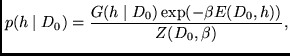 |
(6) |
 |
(7) |
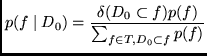
For theoretical purposes, assume we know ![]() and may
use it for learning.
To learn, we use the same distribution
and may
use it for learning.
To learn, we use the same distribution
![]() as above
(prior belief in some hypotheses
as above
(prior belief in some hypotheses ![]() is based exclusively
on the training set).
There is a reason why
we do not use
is based exclusively
on the training set).
There is a reason why
we do not use ![]() instead:
instead:
![]() does not allow
for making a distinction between a better prior belief
in hypotheses
and a better approximation of the test set data.
However, we are interested
in how
does not allow
for making a distinction between a better prior belief
in hypotheses
and a better approximation of the test set data.
However, we are interested
in how ![]() performs on the test set data
performs on the test set data
![]() .
We obtain
.
We obtain
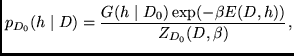 |
(8) |
 |
(9) |
Expected extended
generalization error.
We define the expected extended
generalization error
![]() on the unseen test exemplars
on the unseen test exemplars
![]() :
:
 |
(10) |
Overfitting and underfitting error.
Let us separate the generalization error into an overfitting error ![]() and an
underfitting error
and an
underfitting error ![]() (in analogy to
Wang et al., 1994;
and Guyon et al., 1992).
We will see that
overfitting and underfitting error correspond to the two
different error terms in our algorithm:
decreasing one term is equivalent to decreasing
(in analogy to
Wang et al., 1994;
and Guyon et al., 1992).
We will see that
overfitting and underfitting error correspond to the two
different error terms in our algorithm:
decreasing one term is equivalent to decreasing ![]() ,
decreasing the other is equivalent to decreasing
,
decreasing the other is equivalent to decreasing ![]() .
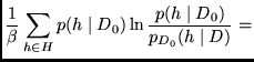
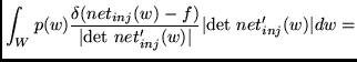
Using the Kullback-Leibler distance (Kullback, 1959),
we measure the information
conveyed by
.
Using the Kullback-Leibler distance (Kullback, 1959),
we measure the information
conveyed by ![]() , but not by
, but not by
![]() (see figure 4).
We may view this as information about
(see figure 4).
We may view this as information about ![]() :
since there are more
:
since there are more ![]() which are compatible with
which are compatible with ![]() than there are
than there are ![]() which are compatible with
which are compatible with ![]() ,
,
![]() 's influence on
's influence on
![]() is stronger than its influence on
is stronger than its influence on
![]() .
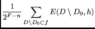
To get the non-stochastic bias (see definition of
.
To get the non-stochastic bias (see definition of ![]() ),
we divide this information by
),
we divide this information by ![]() and obtain the overfitting error:
and obtain the overfitting error:
 |
(11) | ||
 |
|
figure=o.ps,angle=0,width=0.9
|
|
figure=u.ps,angle=0,width=0.9
|
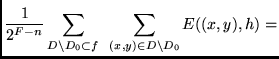
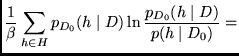
Analogously, we measure the information
conveyed by
![]() , but not by
, but not by ![]() (see figure 5).
This information is about
(see figure 5).
This information is about
![]() .
To get the non-stochastic bias (see definition of
.
To get the non-stochastic bias (see definition of ![]() ),
we divide this information by
),
we divide this information by ![]() and obtain the underfitting error:
and obtain the underfitting error:
 |
(12) | ||
 |
Peaks in ![]() which do not
match peaks of
which do not
match peaks of
![]() produced
by
produced
by
![]() lead to overfitting error.
Peaks of
lead to overfitting error.
Peaks of
![]() produced by
produced by
![]() which do
not match peaks of
which do
not match peaks of ![]() lead to underfitting error.
Overfitting and underfitting error tell us something about the
shape of
lead to underfitting error.
Overfitting and underfitting error tell us something about the
shape of ![]() with respect to
with respect to
![]() , i.e., to
what degree is the prior belief in
, i.e., to
what degree is the prior belief in ![]() compatible with
compatible with
![]() .
.
Why are they called ``overfitting'' and ``underfitting'' error?
Positive contributions to the overfitting error are obtained
where peaks of ![]() do not match
(or are higher than) peaks of
do not match
(or are higher than) peaks of
![]() :
there some
:
there some ![]() will have large probability
after training on
will have large probability
after training on ![]() but will have lower probability after
training on all data
but will have lower probability after
training on all data ![]() .
This is either because
.
This is either because ![]() has been approximated too closely,
or because of sharp peaks in
has been approximated too closely,
or because of sharp peaks in ![]() --
the learning algorithm specializes either on
--
the learning algorithm specializes either on ![]() or
on
or
on ![]() (``overfitting'').
The specialization on
(``overfitting'').
The specialization on ![]() will become even worse if
will become even worse if ![]() is
corrupted by noise -- the case of noisy
is
corrupted by noise -- the case of noisy ![]() will be treated later.
Positive contributions to the underfitting error are obtained
where peaks of
will be treated later.
Positive contributions to the underfitting error are obtained
where peaks of
![]() do not match (or are higher than)
peaks of
do not match (or are higher than)
peaks of ![]() : there some
: there some ![]() will have large probability
after training on all data
will have large probability
after training on all data ![]() , but will have lower probability
after training on
, but will have lower probability
after training on ![]() . This is either due to a poor
. This is either due to a poor
![]() approximation (note that
approximation (note that ![]() is almost fully
determined by
is almost fully
determined by ![]() ), or
to insufficient information about
), or
to insufficient information about ![]() conveyed by
conveyed by ![]() (``underfitting'').
Either the algorithm did not
learn ``enough'' of
(``underfitting'').
Either the algorithm did not
learn ``enough'' of ![]() , or
, or ![]() does not tell
us anything about
does not tell
us anything about ![]() .
In the latter case, there is nothing we can do --
we have to focus on the case where we did not learn
enough about
.
In the latter case, there is nothing we can do --
we have to focus on the case where we did not learn
enough about ![]() .
.
Analysis of overfitting and underfitting error.
![]() holds.
Note: for zero temperature limit
holds.
Note: for zero temperature limit
![]() we obtain
we obtain
![]() and
and
![]() .
.
![]() .
.
![]() , i.e., there is no underfitting error.
For
, i.e., there is no underfitting error.
For
![]() (full stochasticity) we get
(full stochasticity) we get
![]() and
and ![]() (recall that
(recall that ![]() is not the conventional but the
extended expected generalization error).
is not the conventional but the
extended expected generalization error).
Since ![]() ,
,
![]() holds.
In what follows, averages after learning on
holds.
In what follows, averages after learning on ![]() are denoted by
are denoted by ![]() ,
and averages after learning on
,
and averages after learning on ![]() are denoted by
are denoted by ![]() .
.
Since
![]() , we have
, we have
![]() .
.
Analogously, we have
![]() .
.
Thus,
![]() , and
, and
![]() .2With large
.2With large ![]() , after learning on
, after learning on ![]() ,
,
![]() measures the difference between average test set error
and a minimal test set error.
With large
measures the difference between average test set error
and a minimal test set error.
With large ![]() ,
after learning on
,
after learning on ![]() ,
,
![]() measures the difference between average test set error and a maximal
test set error.
So assume we do have a large
measures the difference between average test set error and a maximal
test set error.
So assume we do have a large ![]() (large enough to exceed the minimum
of
(large enough to exceed the minimum
of
![]() ).
We have to assume that
).
We have to assume that ![]() indeed conveys information about the test set:
preferring hypotheses
indeed conveys information about the test set:
preferring hypotheses ![]() with small
with small ![]() by using a larger
by using a larger
![]() leads to smaller test set error
(without this assumption no error decreasing algorithm would
make sense).
leads to smaller test set error
(without this assumption no error decreasing algorithm would
make sense).
![]() can be decreased by enforcing less stochasticity
(by further increasing
can be decreased by enforcing less stochasticity
(by further increasing ![]() ),
but this will increase
),
but this will increase ![]() .
Likewise,
decreasing
.
Likewise,
decreasing ![]() (enforcing more stochasticity)
will decrease
(enforcing more stochasticity)
will decrease ![]() but increase
but increase ![]() .
Increasing
.
Increasing ![]() decreases the
maximal test set error after learning
decreases the
maximal test set error after learning ![]() more than it decreases
the average test set error, thus decreasing
more than it decreases
the average test set error, thus decreasing ![]() , and vice versa.
Decreasing
, and vice versa.
Decreasing ![]() increases the
minimal test set error after learning
increases the
minimal test set error after learning ![]() more than it increases
the average test set error, thus decreasing
more than it increases
the average test set error, thus decreasing ![]() , and vice versa.
This is the above-mentioned
trade-off between stochasticity and
fitting the training set, governed by
, and vice versa.
This is the above-mentioned
trade-off between stochasticity and
fitting the training set, governed by ![]() .
.
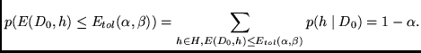
Tolerable error level / Set of acceptable minima.
Let us implicitly define a tolerable error level
![]() which, with confidence
which, with confidence ![]() ,
is the upper bound of the
training set error after learning.
,
is the upper bound of the
training set error after learning.
We would like to have an
algorithm decreasing (1) training set
error (this corresponds to decreasing underfitting error),
and (2) an additional error term, which
should be designed to ensure low overfitting error, given a
fixed small ![]() .
The remainder of this section will lead to an answer for
the question:
how to design this additional error term?
Since low underfitting is obtained by selecting a
hypothesis from
.
The remainder of this section will lead to an answer for
the question:
how to design this additional error term?
Since low underfitting is obtained by selecting a
hypothesis from ![]() , in what follows we will
focus on
, in what follows we will
focus on ![]() only.
Using an appropriate choice of prior belief,
at the end of this section, we
will finally see
that the overfitting error can be reduced by
an error term expressing preference for flat nets.
only.
Using an appropriate choice of prior belief,
at the end of this section, we
will finally see
that the overfitting error can be reduced by
an error term expressing preference for flat nets.
Relative overfitting error.
Let us formally define the relative overfitting error ![]() ,
which is the relative contribution of some
,
which is the relative contribution of some ![]() to the mean
overfitting error of hypotheses set
to the mean
overfitting error of hypotheses set ![]() :
:
| (14) |
 |
(15) |
For ![]() ,
we approximate
,
we approximate
![]() as follows. We
assume that
as follows. We
assume that ![]() is large where
is large where ![]() is large
(trade-off between low
is large
(trade-off between low ![]() and
and ![]() ).
Then
).
Then
![]() has large values (due to large
has large values (due to large ![]() ) where
) where
![]() (assuming
(assuming
![]() is small). We get
is small). We get
![]() . The relative overfitting error can now be approximated by
. The relative overfitting error can now be approximated by
Prior belief in ![]() and
and ![]() .
Assume
.
Assume ![]() was obtained from a
target function
was obtained from a
target function ![]() .
Let
.
Let ![]() be the prior on targets
and
be the prior on targets
and ![]() the
probability of obtaining
the
probability of obtaining ![]() with a given
with a given ![]() . We have
. We have
The data is drawn from a target function with added noise (the noise-free case is treated below). We don't make any assumptions about the nature of the noise -- it does not have to be Gaussian (like, e.g., in MacKay's work, 1992b).
We want to select a ![]() which makes
which makes ![]() small, i.e., those
small, i.e., those
![]() with small
with small
![]() should have high probabilities
should have high probabilities ![]() .
.
We don't know
![]() during learning.
during learning.
![]() is assumed to be drawn from a target
is assumed to be drawn from a target ![]() .
We compute the expectation of
.
We compute the expectation of ![]() , given
, given ![]() .
The probability of the test set
.
The probability of the test set
![]() , given
, given ![]() , is
, is
 |
(19) |
The expected relative overfitting error
![]() is obtained by inserting
equation (20) into equation
(17):
is obtained by inserting
equation (20) into equation
(17):
Minimizing expected relative overfitting error.
We define a
![]() such that
such that
![]() has its largest value near
small expected test set error
has its largest value near
small expected test set error ![]() (see (17)
and (20)).
This definition leads to a low expectation of
(see (17)
and (20)).
This definition leads to a low expectation of
![]() (see equation (21)).
Define
(see equation (21)).
Define
Using equation (20) we get
![]() determines the hypothesis
determines the hypothesis ![]() from
from ![]() that leads to lowest expected test set error.
Consequently, we achieve the lowest expected relative overfitting
error.
that leads to lowest expected test set error.
Consequently, we achieve the lowest expected relative overfitting
error.
![]() helps us to define
helps us to define ![]() :
:
To appreciate the importance of the prior ![]() in the definition of
in the definition of ![]() (see also equation (29)), in what follows,
we will focus on the noise-free case.
(see also equation (29)), in what follows,
we will focus on the noise-free case.
The special case of noise-free data.
Let ![]() be equal to
be equal to
![]() (up to
an normalizing constant):
(up to
an normalizing constant):
From (27) and (17), we obtain
the expected
![]() :
:
For
![]() we obtain in this noise free case
we obtain in this noise free case
The lowest expected test set error
measured by
![]() .
See equation (27).
.
See equation (27).
Noisy data and noise-free data: conclusion.
For both the noise-free and the noisy case,
equation (18) shows that
given ![]() and
and ![]() , the expected test set error depends on
prior target probability
, the expected test set error depends on
prior target probability ![]() .
.
Choice of prior belief.
Now we select some ![]() , our prior belief in target
, our prior belief in target ![]() .
We introduce a formalism similar to Wolpert's
(Wolpert, 1994a ).
.
We introduce a formalism similar to Wolpert's
(Wolpert, 1994a ).
![]() is defined as the probability of obtaining
is defined as the probability of obtaining ![]() by
choosing a
by
choosing a ![]() randomly according to
randomly according to ![]() .
.
Let us first have a look at Wolpert's formalism:
![]() .
By restricting
.
By restricting ![]() to
to ![]() , he obtains an injective function
, he obtains an injective function
![]() ,
which is
,
which is ![]() restricted to
restricted to ![]() .
.
![]() is surjective (because
is surjective (because ![]() is surjective):
is surjective):
 |
(30) | ||
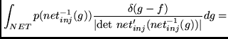 |
|||
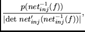 |
However, we prefer to follow another path. Our algorithm (flat minimum
search) tends to prune a weight ![]() if
if ![]() is very flat
in
is very flat
in ![]() 's direction. It prefers regions where
's direction. It prefers regions where
![]() (where many weights lead to the same net function).
Unlike Wolpert's approach, ours distinguishes the probabilities of
targets
(where many weights lead to the same net function).
Unlike Wolpert's approach, ours distinguishes the probabilities of
targets ![]() with
with
![]() .
The advantage is:
we do not only search for
.
The advantage is:
we do not only search for ![]() which are flat in one direction
but for
which are flat in one direction
but for ![]() which are flat in many directions (this corresponds
to a higher probability of the corresponding targets).
Define
which are flat in many directions (this corresponds
to a higher probability of the corresponding targets).
Define
| (31) |
 |
(32) |
 |
(33) |
![]() partitions
partitions ![]() into equivalence
classes. To obtain
into equivalence
classes. To obtain ![]() , we compute the
probability of
, we compute the
probability of ![]() being in the equivalence
class
being in the equivalence
class
![]() ,
if randomly chosen according to
,
if randomly chosen according to ![]() .
An equivalence class corresponds to a net function, i.e.,
.
An equivalence class corresponds to a net function, i.e., ![]() maps all
maps all ![]() of an equivalence class to the same
net function.
of an equivalence class to the same
net function.
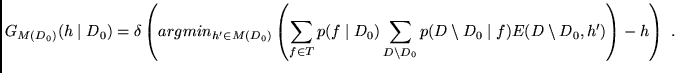
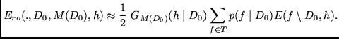
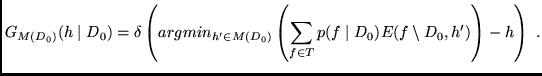
Relation to FMS algorithm.
FMS (from section 3)
works locally in weight space ![]() .
Let
.
Let ![]() be the actual weight vector
found by FMS (with
be the actual weight vector
found by FMS (with ![]() ).
Recall the definition of
).
Recall the definition of
![]() (see (22) and (23)):
we want to find a hypothesis
(see (22) and (23)):
we want to find a hypothesis ![]() which best approximates
those
which best approximates
those ![]() with large
with large ![]() (the test data has high probability of being drawn from such
targets).
We will see that those
(the test data has high probability of being drawn from such
targets).
We will see that those ![]() with
flat
with
flat ![]() locally have high probability
locally have high probability ![]() .
Furthermore we will see that a
.
Furthermore we will see that a ![]() close to
close to ![]() with flat
with flat ![]() has flat
has flat ![]() , too.
To approximate such targets
, too.
To approximate such targets ![]() ,
the only thing we can do is find a
,
the only thing we can do is find a ![]() close to many
close to many ![]() with
with ![]() and large
and large ![]() .
To justify this approximation
(see definition of
.
To justify this approximation
(see definition of ![]() while recalling that
while recalling that
![]() ), we assume (1) that the noise
has mean
), we assume (1) that the noise
has mean ![]() , and (2) that small noise is more likely than
large noise (e.g., Gaussian, Laplace, Cauchy distributions).
, and (2) that small noise is more likely than
large noise (e.g., Gaussian, Laplace, Cauchy distributions).
To restrict
![]() to a local range in
to a local range in ![]() ,
we define regions of equal net functions
,
we define regions of equal net functions
![]() .
.
Note:
![]() .
If
.
If ![]() is
flat along long distances in many directions
is
flat along long distances in many directions
![]() ,
then
,
then ![]() has many elements.
Locally in weight space, at
has many elements.
Locally in weight space, at ![]() with
with ![]() , for
, for
![]() we define:
if the minimum
we define:
if the minimum
![]() exists, then
exists, then
![]() , where
, where
![]() is a constant.
If this minimum does not exist, then
is a constant.
If this minimum does not exist, then
![]() .
.
![]() locally approximates
locally approximates ![]() .
During search for
.
During search for ![]() (corresponding to a hypothesis
(corresponding to a hypothesis ![]() ),
to locally decrease
the expected test set error
(see equation (20)),
we want to enter areas where many
large
),
to locally decrease
the expected test set error
(see equation (20)),
we want to enter areas where many
large ![]() are near
are near ![]() in weight space.
We wish to decrease
the test set error, which is caused by drawing data
from highly probable targets
in weight space.
We wish to decrease
the test set error, which is caused by drawing data
from highly probable targets ![]() (those with large
(those with large
![]() ).
We do not know, however, which
).
We do not know, however, which ![]() 's
are mapped to target's
's
are mapped to target's ![]() by
by ![]() .
Therefore, we focus on
.
Therefore, we focus on ![]() (
(![]() near
near ![]() in weight space),
instead of
in weight space),
instead of
![]() .
Assume
.
Assume
![]() is small enough to allow for a Taylor
expansion, and that
is small enough to allow for a Taylor
expansion, and that ![]() is flat in direction
is flat in direction
![]() :
:
![]() ,
where
,
where ![]() is the Hessian of
is the Hessian of ![]() evaluated at
evaluated at ![]() ,
,
![]() , and
, and
![]() (analogously for higher order derivatives). We see: in a small environment
of
(analogously for higher order derivatives). We see: in a small environment
of ![]() , there is flatness in direction
, there is flatness in direction
![]() , too.
Likewise, if
, too.
Likewise, if ![]() is not flat in any direction, this property also
holds within a small environment of
is not flat in any direction, this property also
holds within a small environment of ![]() .
Only near
.
Only near ![]() with flat
with flat ![]() , there may exist
, there may exist ![]() with large
with large ![]() .
Therefore, it is reasonable
to search for a
.
Therefore, it is reasonable
to search for a ![]() with
with ![]() , where
, where ![]() is flat
within a large region. This means to search for
the
is flat
within a large region. This means to search for
the ![]() determined by
determined by
![]() of equation (22).
Since
of equation (22).
Since ![]() ,
,
![]() holds: we search for a
holds: we search for a ![]() living within a large connected
region, where for all
living within a large connected
region, where for all ![]() within this region
within this region
![]() ,
where
,
where ![]() is defined in section 2.
To conclude: we decrease the relative overfitting error
and the underfitting error by searching for a
flat minimum (see definition of flat minima in section
2).
is defined in section 2.
To conclude: we decrease the relative overfitting error
and the underfitting error by searching for a
flat minimum (see definition of flat minima in section
2).
Practical realization of the Gibbs variant.
(1) Select ![]() and
and
![]() , thus
implicitly choosing
, thus
implicitly choosing ![]() .
.
(2) Compute the set ![]() .
.
(3) Assume we know how data is obtained from target ![]() ,
i. e. we know
,
i. e. we know ![]() ,
,
![]() ,
and the prior
,
and the prior ![]() . Then
we can compute
. Then
we can compute
![]() and
and
![]() .
.
(4) Start with ![]() and increase
and increase ![]() until
equation (13) holds. Now we know the
until
equation (13) holds. Now we know the ![]() from
the implicit choice above.
from
the implicit choice above.
(5) Since we know all we need to compute ![]() ,
select some
,
select some ![]() according to this distribution.
according to this distribution.
Three comments on certain FMS limitations.
1. FMS only approximates the Gibbs
variant given by the definition of
![]() (see (22) and (23)).
(see (22) and (23)).
We only locally approximate ![]() in weight space.
If
in weight space.
If ![]() is locally flat around
is locally flat around ![]() then
there exist units or weights which can be given
with low precision (or can be removed).
If there are other weights
then
there exist units or weights which can be given
with low precision (or can be removed).
If there are other weights ![]() with
with ![]() ,
then one may assume that
there are also points in weight space near such
,
then one may assume that
there are also points in weight space near such ![]() where weights can be given with low precision
(think of, e.g., symmetrical exchange of weights and units).
We assume the local approximation of
where weights can be given with low precision
(think of, e.g., symmetrical exchange of weights and units).
We assume the local approximation of ![]() is good.
The most probable targets represented by flat
is good.
The most probable targets represented by flat ![]() are approximated by a hypothesis
are approximated by a hypothesis ![]() which is also
represented by a flat
which is also
represented by a flat ![]() (where
(where ![]() is near
is near
![]() in weight space). To allow for approximation of
in weight space). To allow for approximation of ![]() by
by ![]() , we have to assume that the hypothesis
set
, we have to assume that the hypothesis
set ![]() is dense in the target set
is dense in the target set ![]() .
If
.
If ![]() is flat in many directions then there are many
is flat in many directions then there are many
![]() that share this flatness and are well-approximated
by
that share this flatness and are well-approximated
by ![]() . The only reasonable
thing FMS can do is to make
. The only reasonable
thing FMS can do is to make ![]() as flat as possible
in a large region around
as flat as possible
in a large region around ![]() ,
to approximate the
,
to approximate the ![]() with large prior probability
(recall that
flat regions are approximated by axis-aligned boxes, as
discussed in section 7, paragraph entitled
``Generalized boxes?'').
This approximation
is fine if
with large prior probability
(recall that
flat regions are approximated by axis-aligned boxes, as
discussed in section 7, paragraph entitled
``Generalized boxes?'').
This approximation
is fine if ![]() is smooth enough in ``unflat'' directions
(small changes in
is smooth enough in ``unflat'' directions
(small changes in ![]() should not result in quite different
net functions).
should not result in quite different
net functions).
2.
Concerning point (3) above:
![]() depends on
depends on
![]() (how the training data is drawn from the
target, see (18)).
(how the training data is drawn from the
target, see (18)).
![]() depends on
depends on
![]() and
and
![]() (how the test data is drawn from the target).
Since we do not know how the data is obtained,
the quality of the approximation of the Gibbs algorithm
may suffer
from noise which has not mean
(how the test data is drawn from the target).
Since we do not know how the data is obtained,
the quality of the approximation of the Gibbs algorithm
may suffer
from noise which has not mean ![]() , or from
large noise being more
probable than small noise.
, or from
large noise being more
probable than small noise.
Of course, if the choice of prior belief does not
match the true target distribution, the quality
of
![]() 's approximation
will suffer as well.
's approximation
will suffer as well.
3.
Concerning point (5) above:
FMS outputs only a single ![]() instead of
instead of ![]() .
This issue is discussed in section 7 (paragraph
entitled ``multiple initializations?'').
.
This issue is discussed in section 7 (paragraph
entitled ``multiple initializations?'').
To conclude:
Our FMS algorithm from section 3 only
approximates the Gibbs algorithm variant. Two
important assumptions are made:
The first is that an appropriate choice of prior belief
has been made.
The second is that the noise on the data is
not too ``weird'' (mean ![]() , small noise more likely).
The two assumptions are necessary for any
algorithm based on an additional error term
besides the training error.
The approximations are:
, small noise more likely).
The two assumptions are necessary for any
algorithm based on an additional error term
besides the training error.
The approximations are: ![]() is approximated locally
in weight space, and flat
is approximated locally
in weight space, and flat ![]() are approximated by
flat
are approximated by
flat ![]() with
with ![]() near
near ![]() 's.
Our Gibbs variant takes into account
that FMS uses only
's.
Our Gibbs variant takes into account
that FMS uses only ![]() for computing flatness.
for computing flatness.