


Next: 4. CONCLUSION
Up: selfref
Previous: 2.1. `SELF-REFERENTIAL' DYNAMICS AND
The following algorithm1for minimizing
 is partly inspired by (but more complex
than) conventional
recurrent network algorithms
(e.g. Robinson and Fallside [2]).
is partly inspired by (but more complex
than) conventional
recurrent network algorithms
(e.g. Robinson and Fallside [2]).
Derivation of the algorithm.
We use the chain rule to compute weight increments
(to be performed after each training sequence)
for all initial weights
 according to
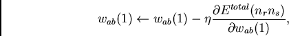 |
(5) |
where  is a constant positive `learning rate'. Thus we obtain
an exact gradient-based algorithm for minimizing
under the `self-referential' dynamics given by (1)-(4).
To reduce writing effort, I introduce some short-hand notation
partly inspired by Williams
[7].
For all units
is a constant positive `learning rate'. Thus we obtain
an exact gradient-based algorithm for minimizing
under the `self-referential' dynamics given by (1)-(4).
To reduce writing effort, I introduce some short-hand notation
partly inspired by Williams
[7].
For all units  and all weights
  ,
,  we write
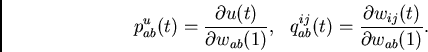 |
(6) |
To begin with, note that
 |
(7) |
Therefore, the remaining problem is to compute
the
 , which can be done by incrementally
computing all
, which can be done by incrementally
computing all
 and
and
 , as we will see.
We have
, as we will see.
We have
 |
(8) |
![\begin{displaymath}
\times
2 \sum_m (ana_m(t) - adr_m(w_{ij})) p_{ab}^{ana_m}(t)
~~]~
~~\}
\end{displaymath}](img67.png) |
(9) |
(where
 is the
  -th bit of 's address),
 |
(10) |
where
 |
(11) |
![\begin{displaymath}
+ 2 \bigtriangleup(t-1)~
g'(\Vert mod(t-1) - adr(w_{ij})\Ver...
...es
\sum_m
[mod_m(t-1) - adr_m(w_{ij})]
p_{ab}^{mod_m}(t-1) .
\end{displaymath}](img73.png) |
(12) |
According to (8)-(12),
the  and
can be updated incrementally at each time step.
This implies that
(5) can be updated incrementally at each time step, too.
The storage complexity is independent
of the sequence length and equals
and
can be updated incrementally at each time step.
This implies that
(5) can be updated incrementally at each time step, too.
The storage complexity is independent
of the sequence length and equals
 . The
computational complexity per time step (of sequences with arbitrary
length) is
. The
computational complexity per time step (of sequences with arbitrary
length) is
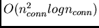 .
.
Next: 4. CONCLUSION
Up: selfref
Previous: 2.1. `SELF-REFERENTIAL' DYNAMICS AND
Juergen Schmidhuber
2003-02-21
Back to Metalearning page
Back to Recurrent Neural Networks page
