This section will show that ALS can use experience to significantly reduce average search time consumed by successive LS calls in cases where there are more and more complex tasks to solve (inductive transfer), and that ALS can be further improved by plugging it into SSA.
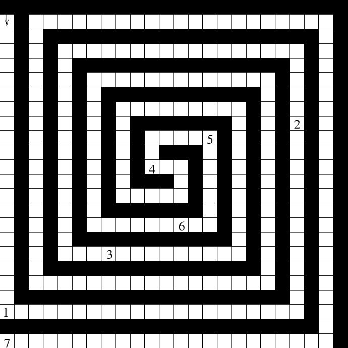
Task. Figure 2 shows a ![]() maze and 7
different goal positions marked 1,2,...,7. With a given goal, the task
is to reach it from the start state. Each goal is further away from
start than goals with lower numbers. We create 4 different ``goalsets''
maze and 7
different goal positions marked 1,2,...,7. With a given goal, the task
is to reach it from the start state. Each goal is further away from
start than goals with lower numbers. We create 4 different ``goalsets''
 ,
, ![]() ,
, ![]() ,
, ![]() .
. ![]() contains goals 1, 2, ..., 3 + i.
One simulation consists of 40 ``epochs''
contains goals 1, 2, ..., 3 + i.
One simulation consists of 40 ``epochs'' ![]() ,
, ![]() , ...
, ... ![]() .
During epochs
.
During epochs
![]() to
to ![]() , all goals in
, all goals in ![]()
![]() have to be found in order of their distances to the start.
Finding a goal yields reward 1.0 divided by solution path length (short
paths preferred). There is no negative reward for collisions.
During each epoch, we update the probability matrices
have to be found in order of their distances to the start.
Finding a goal yields reward 1.0 divided by solution path length (short
paths preferred). There is no negative reward for collisions.
During each epoch, we update the probability matrices ![]() ,
, ![]() and
and
![]() whenever a goal is found
(for all epochs dealing with goalset
whenever a goal is found
(for all epochs dealing with goalset ![]() there are
there are ![]() updates).
For each epoch we store the total
number of steps required to find all goals in the corresponding goalset.
We compare two variants of incremental learning, METHOD 1 and METHOD 2:
updates).
For each epoch we store the total
number of steps required to find all goals in the corresponding goalset.
We compare two variants of incremental learning, METHOD 1 and METHOD 2:
![]()
Comparison. We compare LS by itself, ALS by itself, and SSA+ALS,
for both METHODs 1 and 2.
LS results. Using ![]() and
and 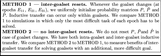 , LS needed
 ![]() time steps to find goal 7 (without any kind of incremental learning
or inductive transfer).
time steps to find goal 7 (without any kind of incremental learning
or inductive transfer).
Learning rate influence. To find optimal learning rates minimizing
the total number of steps during simulations of ALS and SSA+ALS, we tried
all learning rates ![]() in {0.01, 0.02,..., 0.95}. We found that
SSA+ALS is fairly learning rate independent: it solves all tasks
with all learning rates in acceptable time (
in {0.01, 0.02,..., 0.95}. We found that
SSA+ALS is fairly learning rate independent: it solves all tasks
with all learning rates in acceptable time (![]() time steps),
whereas for ALS without SSA (and METHOD 2) only small learning rates are feasible
- large learning rate subspaces do not work for many goals. Thus, the
first type of SSA-generated speed-up lies in the lower expected search
time for appropriate learning rates.
time steps),
whereas for ALS without SSA (and METHOD 2) only small learning rates are feasible
- large learning rate subspaces do not work for many goals. Thus, the
first type of SSA-generated speed-up lies in the lower expected search
time for appropriate learning rates.
With METHOD 1, ALS performs best with a fixed learning rate ![]() , and SSA+ALS performs best with
, and SSA+ALS performs best with ![]() , with additional
uniform noise in
, with additional
uniform noise in
![]() (noise tends to improve SSA+ALS's
performance a little bit, but worsens ALS' performance). With METHOD
2, ALS performs best with
(noise tends to improve SSA+ALS's
performance a little bit, but worsens ALS' performance). With METHOD
2, ALS performs best with
![]() , and SSA+ALS performs best
with
, and SSA+ALS performs best
with ![]() and added noise in
and added noise in
![]() .
.
| Algorithm | METHOD | SET 1 | SET 2 | SET 3 | SET 4 | |
| LS last goal | 4.3 | 1,014 | 9,505 | 17,295 | ||
| LS | 8.7 | 1,024 | 10,530 | 27,820 | ||
| ALS | 1 | 12.9 | 382 | 553 | 650 | |
| SSA + ALS | 1 | 12.2 | 237 | 331 | 405 | |
| ALS | 2 | 13.0 | 487 | 192 | 289 | |
| SSA + ALS | 2 | 11.5 | 345 | 85 | 230 | |
For METHODs 1 and 2 and all goalsets ![]() (
(![]() ), Table
1 lists the numbers of steps required by LS, ALS, SSA+ALS
to find all of
), Table
1 lists the numbers of steps required by LS, ALS, SSA+ALS
to find all of ![]() 's goals during epoch
's goals during epoch
![]() , in which
the agent encounters the goal positions in the goalset for the first time.
, in which
the agent encounters the goal positions in the goalset for the first time.
ALS versus LS. ALS performs much better than LS on goalsets
![]() . ALS does not help to to improve performance on 's
goalset, though (epoch
. ALS does not help to to improve performance on 's
goalset, though (epoch ![]() ), because there are many easily discoverable
programs solving the first few goals.
), because there are many easily discoverable
programs solving the first few goals.
SSA+ALS versus ALS. SSA+ALS always outperforms ALS by itself. For optimal learning rates, the speed-up factor for METHOD 1 ranges from 6 % to 67 %. The speed-up factor for METHOD 2 ranges from 13 % to 26 %. Recall, however, that there are many learning rates where ALS by itself completely fails, while SSA+ALS does not. SSA+ALS is more robust.
Example of bias shifts undone. For optimal learning rates, the
biggest speed-up occurs for ![]() . Here SSA decreases search costs
dramatically: after goal 5 is found, the policy ``overfits''
in the sense that it is too much biased towards problem 5's optimal
(lowest complexity) solution: (1) Repeat step forward until blocked,
rotate left. (2) Jump (1,11). (3) Repeat step forward until blocked,
rotate right. (4) Repeat step forward until blocked, rotate right.
Problem 6's optimal solution can be obtained from this by replacing
the final instruction
by (4) Jump (3,3). This represents a significant
change though (3 probability distributions) and requires time.
Problem 5, however, can also be solved
by replacing its lowest complexity solution's
final instruction by (4) Jump (3,1).
This increases complexity but makes learning problem 6 easier, because
less change is required. After problem 5 has been solved using
the lowest complexity solution, SSA eventually suspects
``overfitting'' because too much computation time goes by without
sufficient new rewards. Before discovering goal 6, SSA undoes apparently
harmful probability shifts until SSC is satisfied again. This makes
Jump instructions more likely and speeds up the search for
a solution to problem 6.
. Here SSA decreases search costs
dramatically: after goal 5 is found, the policy ``overfits''
in the sense that it is too much biased towards problem 5's optimal
(lowest complexity) solution: (1) Repeat step forward until blocked,
rotate left. (2) Jump (1,11). (3) Repeat step forward until blocked,
rotate right. (4) Repeat step forward until blocked, rotate right.
Problem 6's optimal solution can be obtained from this by replacing
the final instruction
by (4) Jump (3,3). This represents a significant
change though (3 probability distributions) and requires time.
Problem 5, however, can also be solved
by replacing its lowest complexity solution's
final instruction by (4) Jump (3,1).
This increases complexity but makes learning problem 6 easier, because
less change is required. After problem 5 has been solved using
the lowest complexity solution, SSA eventually suspects
``overfitting'' because too much computation time goes by without
sufficient new rewards. Before discovering goal 6, SSA undoes apparently
harmful probability shifts until SSC is satisfied again. This makes
Jump instructions more likely and speeds up the search for
a solution to problem 6.
METHOD 1 versus METHOD 2. METHOD 2 works much better than METHOD
1 on ![]() and
and ![]() , but not as well on
, but not as well on ![]() (for both methods
are equal -- differences in performance can be explained by different
learning rates which were optimized for the total task). Why? Optimizing
a policy for goals 1--4 will not necessarily help to speed up discovery
of goal 5, but instead cause a harmful bias shift by overtraining the
probability matrices. METHOD 1, however, can extract enough useful
knowledge from the first 4 goals to decrease search costs for goal 5.
(for both methods
are equal -- differences in performance can be explained by different
learning rates which were optimized for the total task). Why? Optimizing
a policy for goals 1--4 will not necessarily help to speed up discovery
of goal 5, but instead cause a harmful bias shift by overtraining the
probability matrices. METHOD 1, however, can extract enough useful
knowledge from the first 4 goals to decrease search costs for goal 5.
|
More SSA benefits. Table 2 lists the number of steps
consumed during the final epoch ![]() of each goalset
of each goalset ![]() (the results
of LS by itself are identical to those in table 1).
Using SSA typically improves the final result, and never worsens it.
Speed-up factors range from 0 to 560 %.
(the results
of LS by itself are identical to those in table 1).
Using SSA typically improves the final result, and never worsens it.
Speed-up factors range from 0 to 560 %.
|
For all goalsets Table 3 lists the total number of
steps consumed during all epochs of one simulation, the total number of
all steps for those epochs (![]() ,
, ![]() ,
, ![]() ,
, ![]() ) in which
new goalsets are introduced, and the total number of steps required for
the final epochs (
) in which
new goalsets are introduced, and the total number of steps required for
the final epochs (![]() ,
, ![]() ,
, ![]() ,
, ![]() ). SSA always
improves the results. For the total number of steps -- which is an
almost linear function of the time consumed during the simulation -- the
SSA-generated speed-up is 60% for METHOD 1 and 108 % for METHOD 2 (the
``fully incremental'' method). Although METHOD 2 speeds up performance
during each goalset's first epoch (ignoring the costs that occurred before
introduction of this goalset),
final results are better without inter-goalset learning.
This is not so surprising: by using policies optimized for previous
goalsets, we generate bias
shifts for speeding up discovery of new, acceptable solutions, without
necessarily making optimal solutions of future tasks more likely
(due to ``evolutionary ballast'' from previous solutions).
). SSA always
improves the results. For the total number of steps -- which is an
almost linear function of the time consumed during the simulation -- the
SSA-generated speed-up is 60% for METHOD 1 and 108 % for METHOD 2 (the
``fully incremental'' method). Although METHOD 2 speeds up performance
during each goalset's first epoch (ignoring the costs that occurred before
introduction of this goalset),
final results are better without inter-goalset learning.
This is not so surprising: by using policies optimized for previous
goalsets, we generate bias
shifts for speeding up discovery of new, acceptable solutions, without
necessarily making optimal solutions of future tasks more likely
(due to ``evolutionary ballast'' from previous solutions).
LS by itself needs ![]() steps for finding all goals
in
steps for finding all goals
in ![]() . Recall that
. Recall that ![]() of them are spent for finding
only goal 7. Using inductive transfer, however, we obtain large
speed-up factors. METHOD 1 with SSA+ALS improves performance by a
factor in excess of 40 (see results of SSA+ALS on the first epoch
of
of them are spent for finding
only goal 7. Using inductive transfer, however, we obtain large
speed-up factors. METHOD 1 with SSA+ALS improves performance by a
factor in excess of 40 (see results of SSA+ALS on the first epoch
of ![]() ). Figure 3(A) plots performance against
epoch numbers. Each time the goalset changes, initial search costs
are large (reflected by sharp peaks). Soon, however, both methods
incorporate experience into the policy. We see that SSA keeps initial
search costs significantly lower.
). Figure 3(A) plots performance against
epoch numbers. Each time the goalset changes, initial search costs
are large (reflected by sharp peaks). Soon, however, both methods
incorporate experience into the policy. We see that SSA keeps initial
search costs significantly lower.
The safety net effect. Figure 3(B) plots epoch numbers against average probability of programs computing solutions. With METHOD 1, SSA+ALS tends to keep the probabilities lower than ALS by itself: high program probabilities are not always beneficial. With METHOD 2, SSA undoes many policy modifications when goalsets change, thus keeping the policy flexible and reducing initial search costs.
Effectively, SSA is controlling the prior on the search space such that
overall average search time is reduced, given a particular task sequence.
For METHOD 1, after ![]() the number of still valid modifications of
policy components (probability distributions) is 377 for ALS, but only
61 for SSA+ALS (therefore, 61 is SSA+ALS's total final stack size).
For METHOD 2, the corresponding numbers are 996 and 63. We see that
SSA keeps only about 16% respectively 6% of all modifications.
The remaining modifications are deemed unworthy because they have
not been observed to trigger lifelong reward speed-ups.
Clearly, SSA prevents ALS from overdoing its policy modifications
(``safety net effect''). This is SSA's simple, basic purpose: undo
certain learning algorithms' policy changes and bias shifts once they
start looking harmful in terms of long-term reward/time ratios.
the number of still valid modifications of
policy components (probability distributions) is 377 for ALS, but only
61 for SSA+ALS (therefore, 61 is SSA+ALS's total final stack size).
For METHOD 2, the corresponding numbers are 996 and 63. We see that
SSA keeps only about 16% respectively 6% of all modifications.
The remaining modifications are deemed unworthy because they have
not been observed to trigger lifelong reward speed-ups.
Clearly, SSA prevents ALS from overdoing its policy modifications
(``safety net effect''). This is SSA's simple, basic purpose: undo
certain learning algorithms' policy changes and bias shifts once they
start looking harmful in terms of long-term reward/time ratios.
It should be clear that the SSA+ALS implementation is just one of many possible SSA applications -- we may plug many alternative learning algorithms into the basic cycle.