The explorer's life in environment ![]() lasts
from time 0 (birth) to unknown time
lasts
from time 0 (birth) to unknown time ![]() (death).
Two
(death).
Two ![]() matrices
(
matrices
(![]() and
and ![]() )
of modifiable real values represent
the learner's modules.
)
of modifiable real values represent
the learner's modules. ![]() 's
's ![]() -th variable, vector-valued column is denoted
-th variable, vector-valued column is denoted ![]() ;
its
;
its ![]() -th real-valued component
-th real-valued component
![]() ; similarly for
; similarly for
![]() .
A variable InstructionPointer (IP)
with range
.
A variable InstructionPointer (IP)
with range
![]() always points
to one of the module pair's columns.
always points
to one of the module pair's columns.
![]() is the learner's variable internal state with
is the learner's variable internal state with ![]() -th
component
-th
component ![]()
![]()
![]()
![]() for
for
![]() .
.
Throughout its life the learner repeats the following
basic cycle over and over:
select and execute
instruction ![]()
![]() with probability
with probability ![]() (here
(here ![]() denotes a set of
possible instructions), where
denotes a set of
possible instructions), where
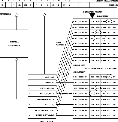 |
Reward.
Occasionally ![]() may distribute real-valued external reward
equally between both modules.
may distribute real-valued external reward
equally between both modules.
![]() is each module's cumulative external
reward obtained between time 0 and time
is each module's cumulative external
reward obtained between time 0 and time ![]() , where
, where ![]() .
In addition there may be occasional
surprise rewards triggered by
the special instruction Bet!(x,y,c,d)
.
In addition there may be occasional
surprise rewards triggered by
the special instruction Bet!(x,y,c,d)
![]()
![]() .
Suppose the two modules have agreed on executing a Bet! instruction,
given a certain IP value. The probabilities of its four
arguments
.
Suppose the two modules have agreed on executing a Bet! instruction,
given a certain IP value. The probabilities of its four
arguments
![]() and
and
![]() depend on both modules: the arguments are selected
according to the four probability distributions
depend on both modules: the arguments are selected
according to the four probability distributions
![]() ,
, ![]() ,
, ![]() ,
, ![]() (details in the appendix).
If
(details in the appendix).
If ![]() then no module will be rewarded.
then no module will be rewarded.
![]() means that
means that ![]() bets on
bets on ![]()
![]()
![]() ,
while
,
while ![]() bets on
bets on ![]()
![]()
![]() .
.
![]() means that
means that ![]() bets on
bets on ![]()
![]()
![]() ,
while
,
while ![]() bets on
bets on ![]()
![]()
![]() .
Execution of the instruction will result in an immediate test:
which module is wrong, which is right?
The former will be punished (surprise reward minus 1),
the other one will be rewarded (
.
Execution of the instruction will result in an immediate test:
which module is wrong, which is right?
The former will be punished (surprise reward minus 1),
the other one will be rewarded (![]() ).
Note that in this particular implementation the modules always
bet a fixed amount of 1 -- alternative implementations, however,
may compute real-valued bids via appropriate instruction sequences.
).
Note that in this particular implementation the modules always
bet a fixed amount of 1 -- alternative implementations, however,
may compute real-valued bids via appropriate instruction sequences.
Interpretation of surprise rewards.
Instructions are likely to be executed only if both modules
collectively assign them high conditional probabilities,
given ![]() and
and ![]() .
In this sense both must ``agree''
on each executed instruction of the lifelong computation process.
In particular,
both collectively set arguments
.
In this sense both must ``agree''
on each executed instruction of the lifelong computation process.
In particular,
both collectively set arguments ![]() in the case they
decide to execute a Bet! instruction. By setting
in the case they
decide to execute a Bet! instruction. By setting ![]() they express that their predictions of the Bet! outcome differ.
Hence
they express that their predictions of the Bet! outcome differ.
Hence ![]() will be rewarded for
luring
will be rewarded for
luring ![]() into agreeing upon instruction subsequences
(algorithms)
that include Bet! instructions demonstrating that certain
calculations yield results different from
what
into agreeing upon instruction subsequences
(algorithms)
that include Bet! instructions demonstrating that certain
calculations yield results different from
what ![]() expects, and vice versa.
Thus each module is motivated to discover algorithms whose
outcomes surprise the other;
but each also may reduce the probability of
algorithms it does not expect to surprise the other.
expects, and vice versa.
Thus each module is motivated to discover algorithms whose
outcomes surprise the other;
but each also may reduce the probability of
algorithms it does not expect to surprise the other.
The sheer existence of the Bet! instruction motivates each module to act not only to receive external reward but also to obtain surprise reward, by discovering algorithmic regularities the other module still finds surprising -- a type of curiosity.
Trivial and random results.
Why not provide reward if ![]()
![]()
![]() and
and
![]() (meaning both modules
rightly believe in
(meaning both modules
rightly believe in ![]()
![]()
![]() )?
Because then both would soon focus on this particular way of
making a correct and rewarding prediction, and do nothing else.
Why not provide punishment if
)?
Because then both would soon focus on this particular way of
making a correct and rewarding prediction, and do nothing else.
Why not provide punishment if ![]()
![]()
![]() and
and
![]() (meaning that both modules are wrong)?
Because then both modules would soon be discouraged from
making any prediction at all.
In case
(meaning that both modules are wrong)?
Because then both modules would soon be discouraged from
making any prediction at all.
In case ![]() the truth of
the truth of ![]()
![]()
![]() is considered a
well-known, ``trivial'' fact whose confirmation does not deserve reward.
In case
is considered a
well-known, ``trivial'' fact whose confirmation does not deserve reward.
In case ![]() the truth of
the truth of ![]()
![]()
![]() is
considered a subjectively ``random,'' irregular result.
Surprise rewards
can occur only in the case both modules' opinions differ.
They reflect one module's disappointed confident expectation,
and the other's justified one,
where, by definition, ``confidence'' translates into ``agreement on the
surprising instruction sequence'' --
no surprise without such confidence.
is
considered a subjectively ``random,'' irregular result.
Surprise rewards
can occur only in the case both modules' opinions differ.
They reflect one module's disappointed confident expectation,
and the other's justified one,
where, by definition, ``confidence'' translates into ``agreement on the
surprising instruction sequence'' --
no surprise without such confidence.
Examples of learnable regularities.
A Turing-equivalent instruction set
![]() (one that permits construction of a
universal Turing machine) allows
exploitation of arbitrary computable regularities
[11,2,39,14]
to trigger or avoid surprises.
For instance, in partially predictable environments the following
types of regularities may help to reliably generate matches of
computational outcomes. (1) Observation/prediction: selected inputs
computed via the environment (observations obtained through ``active
perception'') may match the outcomes of earlier internal computations
(predictions). (2) Observation/explanation: memorized inputs
computed via the environment may match the outcomes of later internal
computations (explanations). (3) Planning/acting: outcomes
of internal computations (planning processes) may match desirable
inputs later computed via the environment (with the help of
environment-changing instructions). (4) ``Internal'' regularities:
the following computations yield matching results --
subtracting 2 from 14, adding 3, 4, and 5, multiplying 2 by 6.
Or: apparently, the computation of the truth value of
``
(one that permits construction of a
universal Turing machine) allows
exploitation of arbitrary computable regularities
[11,2,39,14]
to trigger or avoid surprises.
For instance, in partially predictable environments the following
types of regularities may help to reliably generate matches of
computational outcomes. (1) Observation/prediction: selected inputs
computed via the environment (observations obtained through ``active
perception'') may match the outcomes of earlier internal computations
(predictions). (2) Observation/explanation: memorized inputs
computed via the environment may match the outcomes of later internal
computations (explanations). (3) Planning/acting: outcomes
of internal computations (planning processes) may match desirable
inputs later computed via the environment (with the help of
environment-changing instructions). (4) ``Internal'' regularities:
the following computations yield matching results --
subtracting 2 from 14, adding 3, 4, and 5, multiplying 2 by 6.
Or: apparently, the computation of the truth value of
``![]() is the sum of two primes'' yields the same result
for each even integer
is the sum of two primes'' yields the same result
for each even integer ![]() (Goldbach's conjecture).
(5) Mixtures of (1-4).
For instance, raw inputs may be too noisy to be precisely predictable.
Still, there may be internally computable, predictable, informative input
transformations [33]. For example, hearing the first
two words of the sentence ``John eats chips'' does not make the word
``chips'' predictable, but at least it is likely that the third word will
represent something edible. Examples (1-5) mainly differ in the degree
to which the environment is involved in the computation processes, and
in the temporal order of the computations.
(Goldbach's conjecture).
(5) Mixtures of (1-4).
For instance, raw inputs may be too noisy to be precisely predictable.
Still, there may be internally computable, predictable, informative input
transformations [33]. For example, hearing the first
two words of the sentence ``John eats chips'' does not make the word
``chips'' predictable, but at least it is likely that the third word will
represent something edible. Examples (1-5) mainly differ in the degree
to which the environment is involved in the computation processes, and
in the temporal order of the computations.
Curiosity's utility? The two-module system is supposed to solve self-generated tasks in an unsupervised manner. But can the knowledge collected in this way help to solve externally posed tasks? Intuition suggests that the more one knows about the world the easier it will be to maximize external reward. In fact, later I will present an example where a curious system indeed outperforms a non-curious one. This does not reflect a universal law though: in general there is no guarantee that curiosity will not turn out to be harmful (for example, by ``killing the cat'' [40]).
Relative reward weights?
Let ![]() and
and ![]() denote
denote ![]() 's and
's and ![]() 's
respective total cumulative rewards obtained
between time 0 and time
's
respective total cumulative rewards obtained
between time 0 and time ![]() .
The sum of both modules' surprise rewards always remains zero:
we have
.
The sum of both modules' surprise rewards always remains zero:
we have
![]() for all
for all ![]() .
.
If we adopt the traditional hope that exploration will contribute to accelerating environmental rewards, then zero-sum surprise rewards seem to afford less need to worry about the relative weights of surprise versus other rewards than the surprise rewards of previous approaches, which did not add up to zero.
Enforcing fairness. To avoid situations where one module consistently outperforms the other, the instruction set includes a special LI that copies the currently superior module onto the other (see the appendix for details). This LI (with never-vanishing probability) will occasionally bring both modules on a par with each other.
In principle, each module could learn to outsmart the other by executing
subsequences of instructions that include LIs. But how can we ensure that
each module indeed improves? Note that arithmetic actions affecting ![]() and jump instructions affecting IP cause a highly non-Markovian
setting and prevent traditional RL algorithms based on dynamic
programming from being applicable. For such reasons I use Incremental
Self-improvement (IS) [35,34] to
deal with both modules' complex spatio-temporal credit assignment problem.
and jump instructions affecting IP cause a highly non-Markovian
setting and prevent traditional RL algorithms based on dynamic
programming from being applicable. For such reasons I use Incremental
Self-improvement (IS) [35,34] to
deal with both modules' complex spatio-temporal credit assignment problem.