


Next: SIMULATIONS: IMAGE CODING
Up: EXAMPLE 3: Discovering Factorial
Previous: EXAMPLE 3: Discovering Factorial
In its most simple form,
predictability minimization
is based on a feedforward network with  input units
and
input units
and  output units (or code units).
The
output units (or code units).
The  -th code unit produces
an output value
-th code unit produces
an output value
![$y^p_i \in [0, 1]$](img72.png) in
response to the current external input
vector
in
response to the current external input
vector  .
The central idea is:
For each code unit there is an
adaptive predictor network that tries to predict the code unit
from the remaining
.
The central idea is:
For each code unit there is an
adaptive predictor network that tries to predict the code unit
from the remaining  code units.
But each code unit in turn tries to become
as unpredictable as possible.
The only way it can do so is by representing
environmental properties
that are statistically independent from environmental properties
represented by the remaining code units.
The principle of predictability minimization
was first described in [22].
code units.
But each code unit in turn tries to become
as unpredictable as possible.
The only way it can do so is by representing
environmental properties
that are statistically independent from environmental properties
represented by the remaining code units.
The principle of predictability minimization
was first described in [22].
The predictor network for code unit is
called  . Its output in response to the
 is called
  .
is trained to minimize
.
is trained to minimize
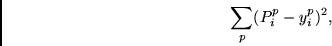 |
(2) |
thus learning to predict the
the conditional expectation
 of
of  , given the set
 .
But the code units try to maximize the same (!) objective function
the predictors try to minimize:
.
But the code units try to maximize the same (!) objective function
the predictors try to minimize:
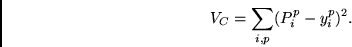 |
(3) |
Predictors and code units co-evolve by fighting
each other. See details in
[22] and especially in
[24].
Let us
assume that the do not get trapped in local minima
and perfectly learn the conditional expectations.
It then turns out that the objective function  (first given in
[22])
is essentially equivalent
to the following one
(also given in [22]):
(first given in
[22])
is essentially equivalent
to the following one
(also given in [22]):
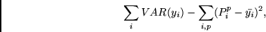 |
(4) |
where  denotes the mean activation of unit ,
and
denotes the mean activation of unit ,
and  denotes the variance operator.
The equivalence of (3) and (4) was observed by
Peter Dayan, Richard Zemel and Alex Pouget (SALK Institute, 1992).
See [24] for details.
(4) gives some intuition about what is going on while
(3) is maximized.
The first term of (4) tends to enforce binary units,
while the second term tends to make the conditional
expectations equal to the unconditional expectations, thus
encouraging statistical independence.
denotes the variance operator.
The equivalence of (3) and (4) was observed by
Peter Dayan, Richard Zemel and Alex Pouget (SALK Institute, 1992).
See [24] for details.
(4) gives some intuition about what is going on while
(3) is maximized.
The first term of (4) tends to enforce binary units,
while the second term tends to make the conditional
expectations equal to the unconditional expectations, thus
encouraging statistical independence.
Note that unlike with many previous approaches to unsupervised learning,
the system is not limited to local ``winner-take-all'' representations.
Instead, there may be distributed code representations
based on many code units that are active simultaneously
- as long as the ``winners''
stand for independent abstract features extracted from the input data.
And unlike previous approaches, the method allows
for discovering nonlinear predictability, and
for nonlinear
pattern transformations to obtain codes with statistically
independent components. Note that
statistical independence implies decorrelation. But decorrelation
does not imply statistical independence.
Next: SIMULATIONS: IMAGE CODING
Up: EXAMPLE 3: Discovering Factorial
Previous: EXAMPLE 3: Discovering Factorial
Juergen Schmidhuber
2003-02-19