The following algorithm for minimizing
![]() is partly inspired by
conventional
recurrent network algorithms
(e.g. [2],
[7]).
The notation is partly inspired by
[8].
is partly inspired by
conventional
recurrent network algorithms
(e.g. [2],
[7]).
The notation is partly inspired by
[8].
Derivation.
Before training, all initial weights
![]() are randomly initialized.
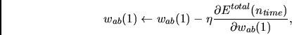
The chain rule serves to compute weight increments
(to be performed after each training sequence)
for all initial weights
according to
are randomly initialized.
The chain rule serves to compute weight increments
(to be performed after each training sequence)
for all initial weights
according to
 |
(5) |
We write
| (6) |
First note that
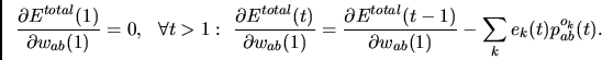 |
(7) |
| (8) |
![\begin{displaymath}
p_{ab}^{y_k}(t+1)= f_{y_k}'(net_{y_k}(t+1)) \sum_l
\frac{\partial}
{\partial w_{ab}(1)} [ l(t)w_{y_kl}(t) ] =
\end{displaymath}](img58.png)
| (9) |
| (10) |
| (11) |
According to equations (8)-(11),
variables holding
the ![]() and
and
![]() values
can be updated incrementally at each time step.
This implies that
(5) can be updated incrementally, too.
With non-degenerate networks,
the algorithm's storage complexity is dominated by the number of
variables for storing the
values
can be updated incrementally at each time step.
This implies that
(5) can be updated incrementally, too.
With non-degenerate networks,
the algorithm's storage complexity is dominated by the number of
variables for storing the
![]() values. This number
is independent
of the sequence length and equals
values. This number
is independent
of the sequence length and equals
![]() . Since
. Since
![]() ,
,
![]() (like with RTRL).
The computational complexity per time step
also is
(like with RTRL).
The computational complexity per time step
also is ![]() - essentially the same as the one of RTRL.
Since
- essentially the same as the one of RTRL.
Since
![]() , however,
, however,
![]() (like with time-efficient BPTT and unlike with RTRL's
much worse
(like with time-efficient BPTT and unlike with RTRL's
much worse
![]() ).
).