Algorithmic complexity theory provides various different but closely related measures for the complexity (or simplicity) of objects. We will focus on the one that appears to be the most useful for machine learning. Informally speaking, the complexity of a computable object is the length of the shortest program that computes it and halts, where the set of possible programs forms a prefix code.
Machine.
To make this more precise, consider a Turing machine (TM) with 3 tapes:
the program tape, the work tape, and the output tape. All three are finite
but may grow indefinitely.
For simplicity, but without loss of generality,
let us focus on binary tape alphabets ![]() .
Initially, the work tape and the output tape consist
of a single square filled with a zero. The program tape consists of
finitely many squares, each filled with a zero or a one.
Each tape has a scanning head. Initially, the scanning head of each
tape points to its first square. The program tape is ``read only,''
the output tape is ``write only'' and their
scanning heads may be shifted only to the right (one square at a time).
The work tape is ``read/write'' and its scanning head may move in
both directions. Whenever the scanning heads of work tape
or output tape shift beyond the current tape boundary,
an additional square is appended and filled with a zero.
The case of the program tape's scanning head shifting beyond the
program tape boundary will be considered later.
For the moment we assume that this does never happen.
The TM has a finite number of internal states (one of them being
the initial state). Its
behavior is specified by a function
.
Initially, the work tape and the output tape consist
of a single square filled with a zero. The program tape consists of
finitely many squares, each filled with a zero or a one.
Each tape has a scanning head. Initially, the scanning head of each
tape points to its first square. The program tape is ``read only,''
the output tape is ``write only'' and their
scanning heads may be shifted only to the right (one square at a time).
The work tape is ``read/write'' and its scanning head may move in
both directions. Whenever the scanning heads of work tape
or output tape shift beyond the current tape boundary,
an additional square is appended and filled with a zero.
The case of the program tape's scanning head shifting beyond the
program tape boundary will be considered later.
For the moment we assume that this does never happen.
The TM has a finite number of internal states (one of them being
the initial state). Its
behavior is specified by a function ![]() (implemented as a
look-up table).
(implemented as a
look-up table). ![]() maps the current state
and the contents of the square above the scanning head of
the work tape to a new state and an action.
There are 8 actions:
shift worktape left/right,
write 1/0 on worktape,
write 1/0 on output tape and shift its scanning head right,
copy contents above scanning head of program tape
onto square above scanning head of work tape and shift program tape's
scanning head right, and halt.
maps the current state
and the contents of the square above the scanning head of
the work tape to a new state and an action.
There are 8 actions:
shift worktape left/right,
write 1/0 on worktape,
write 1/0 on output tape and shift its scanning head right,
copy contents above scanning head of program tape
onto square above scanning head of work tape and shift program tape's
scanning head right, and halt.
Self-delimiting programs.
Let ![]() denote the number of bits in the bitstring
denote the number of bits in the bitstring ![]() .
Consider a non-empty bitstring
.
Consider a non-empty bitstring ![]() written onto the
program tape such that the scanning head points to the first bit of
written onto the
program tape such that the scanning head points to the first bit of ![]() .
.
![]() is a program for some TM
is a program for some TM ![]() , iff
, iff
![]() reads all
reads all ![]() bits and halts.
In other words, during the (eventually terminating) computation process
the head of
bits and halts.
In other words, during the (eventually terminating) computation process
the head of ![]() 's program tape incrementally
moves from its start position to the end of
's program tape incrementally
moves from its start position to the end of ![]() , but not
any further. One may say that
, but not
any further. One may say that
![]() carries in itself the information about when to
stop, and about its own length.
Obviously, no program can be the prefix of another one.
carries in itself the information about when to
stop, and about its own length.
Obviously, no program can be the prefix of another one.
Compiler theorem.
Each TM ![]() , mapping bitstrings (written
onto the program tape) to outputs (written onto the output tape)
computes a partial function
, mapping bitstrings (written
onto the program tape) to outputs (written onto the output tape)
computes a partial function
![]() (
(![]() is undefined if
is undefined if ![]() does not halt).
It is well known that there is a universal TM
does not halt).
It is well known that there is a universal TM ![]() with the
following property:
for every TM
with the
following property:
for every TM ![]() there exists a constant prefix
there exists a constant prefix ![]() such that
such that
![]() for all bitstrings
for all bitstrings ![]() .
The prefix
.
The prefix ![]() is the compiler that compiles programs for
is the compiler that compiles programs for ![]() into
equivalent programs for
into
equivalent programs for ![]() .
.
In what follows, let ![]() denote a (self-delimiting) program.
denote a (self-delimiting) program.
Kolmogorov complexity.
Given ![]() ,
the Kolmogorov complexity (a.k.a. ``algorithmic complexity,''
``algorithmic information,'' or
occasionally ``Kolmogorov-Chaitin complexity'')
of an arbitrary bitstring
,
the Kolmogorov complexity (a.k.a. ``algorithmic complexity,''
``algorithmic information,'' or
occasionally ``Kolmogorov-Chaitin complexity'')
of an arbitrary bitstring ![]() is denoted as
is denoted as ![]() and is defined as
the length of a shortest program producing
and is defined as
the length of a shortest program producing ![]() on
on ![]() :
:
Invariance theorem.
Due to the compiler theorem,
![]() for two universal machines
for two universal machines
![]() and
and ![]() .
Therefore we may choose one particular
universal machine
.
Therefore we may choose one particular
universal machine ![]() and henceforth write
and henceforth write
![]() .
.
Machine learning, MDL, and the prior problem.
In machine learning applications, we are often concerned
with the following problem:
given training data ![]() , we would like to select
the most probable hypothesis
, we would like to select
the most probable hypothesis ![]() generating the data.
Bayes formula yields
generating the data.
Bayes formula yields
| (1) |
| (2) |
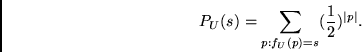
Universal prior.
Define ![]() , the a priori probability of a bitstring
, the a priori probability of a bitstring ![]() ,
as the probability of guessing a (halting) program
that computes
,
as the probability of guessing a (halting) program
that computes ![]() on
on ![]() . Here, the way of guessing is defined
by the following procedure:
initially, the program tape consists of a single square.
Whenever the scanning head of the program tape shifts
to the right, do: (1) Append a new square.
(2) With probability
. Here, the way of guessing is defined
by the following procedure:
initially, the program tape consists of a single square.
Whenever the scanning head of the program tape shifts
to the right, do: (1) Append a new square.
(2) With probability ![]() fill it with a 0;
with probability
fill it with a 0;
with probability ![]() fill it with a 1.
We obtain
fill it with a 1.
We obtain
Under different universal priors (based on different universal
machines), probabilities of a given string
differ by not more than a constant factor independent of the
string size, due to the invariance
theorem (the constant factor corresponds to the probability of
guessing a compiler).
Therefore
we may drop the index ![]() and write
and write ![]() instead of
instead of ![]() .
This justifies the name ``universal prior,''
also known as the Solomonoff-Levin distribution.
.
This justifies the name ``universal prior,''
also known as the Solomonoff-Levin distribution.
Algorithmic entropy.
![]() is denoted by
is denoted by ![]() , the algorithmic entropy of
, the algorithmic entropy of ![]() .
.
Dominance of shortest programs.
It can be shown (the proof is non-trivial) that
| (3) |
Dominance of universal prior.
Suppose there are infinitely many enumerable solution candidates (strings):
amazingly, ![]() dominates all discrete enumerable semimeasures P
(including probability distributions) in the following sense:
for each
dominates all discrete enumerable semimeasures P
(including probability distributions) in the following sense:
for each ![]() there is a constant
there is a constant ![]() such that
such that
![]() for
all strings
for
all strings ![]() .
.
Inductive inference and Occam's razor.
Occam's razor prefers solutions whose minimal descriptions are short over
solutions whose minimal descriptions are longer.
The ``modern'' prefix-based version of
Solomonoff's theory of inductive inference justifies
Occam's razor in the following way.
Suppose the problem is to extrapolate a sequence of symbols
(bits, without loss of generality).
We have already observed a bitstring ![]() and would
like to predict the next bit.
Let
and would
like to predict the next bit.
Let ![]() denote the event ``
denote the event ``![]() is followed by symbol
is followed by symbol ![]() ''
for
''
for ![]() .
Bayes tells us
.
Bayes tells us
Since Kolmogorov complexity is incomputable in general, the universal prior is so, too. A popular myth states that this fact renders useless the concepts of Kolmogorov complexity, as far as practical machine learning is concerned. But this is not so, as will be seen next. There we focus on a natural, computable, yet very general extension of Kolmogorov complexity.
Levin complexity.
Let us slightly extend the notion of a program.
In what follows, a program is
a string on the program tape which can be
scanned completely by ![]() .
The same program may lead to different results,
depending on the runtime.
For a given computable string, consider
the logarithm of the probability of guessing a program
that computes it, plus the logarithm of the corresponding runtime.
The Levin complexity of the string
is the minimal possible value of this.
More formally, let
.
The same program may lead to different results,
depending on the runtime.
For a given computable string, consider
the logarithm of the probability of guessing a program
that computes it, plus the logarithm of the corresponding runtime.
The Levin complexity of the string
is the minimal possible value of this.
More formally, let ![]() scan a program
scan a program ![]() (a program in the extended sense)
written onto the program tape
before it finishes printing
(a program in the extended sense)
written onto the program tape
before it finishes printing ![]() onto the work tape.
Let
onto the work tape.
Let ![]() be the number of steps taken before
be the number of steps taken before ![]() is printed. Then
is printed. Then
Universal search.
Suppose we have got a problem whose solution can be represented
as a (bit)string.
Levin's universal optimal search algorithm essentially generates
and evaluates all
strings (solution candidates) in order of their ![]() complexity,
until a solution is found.
This is essentially equivalent to
enumerating
all programs in order of decreasing probabilities, divided
by their runtimes.
Each program computes a string that
is tested to see whether it is a solution to the given problem.
If so, the search is stopped.
To get some intuition on universal search, let
complexity,
until a solution is found.
This is essentially equivalent to
enumerating
all programs in order of decreasing probabilities, divided
by their runtimes.
Each program computes a string that
is tested to see whether it is a solution to the given problem.
If so, the search is stopped.
To get some intuition on universal search, let ![]() denote the probability of computing a solution
denote the probability of computing a solution ![]() from a halting program
from a halting program ![]() on the program tape. For each
on the program tape. For each ![]() there is a given runtime
there is a given runtime ![]() .
Now suppose the following gambling scenario.
You bet on the success of some
.
Now suppose the following gambling scenario.
You bet on the success of some ![]() . The bid is
. The bid is ![]() .
To minimize your expected losses, you are going to bet on the
.
To minimize your expected losses, you are going to bet on the ![]() with maximal
with maximal
![]() . If you fail to hit
a solution, you may bet again, but not on a
. If you fail to hit
a solution, you may bet again, but not on a ![]() you
already bet on. Continuing this procedure,
you are going to list halting programs
you
already bet on. Continuing this procedure,
you are going to list halting programs ![]() in order of decreasing
in order of decreasing
![]() .
Of course,
neither
.
Of course,
neither ![]() nor
nor ![]() are usually known in advance.
Still, for a broad class of problems,
including inversion problems and
time-limited optimization problems,
universal search
can be shown to be optimal with respect to total expected
search time,
leaving aside a constant factor independent of the problem size.
If string
are usually known in advance.
Still, for a broad class of problems,
including inversion problems and
time-limited optimization problems,
universal search
can be shown to be optimal with respect to total expected
search time,
leaving aside a constant factor independent of the problem size.
If string ![]() can be computed within
can be computed within ![]() time steps
by a program
time steps
by a program ![]() , and the probability of guessing
, and the probability of guessing ![]() (as above) is
(as above) is ![]() ,
then within
,
then within
![]() time steps,
systematic enumeration according to Levin will
generate
time steps,
systematic enumeration according to Levin will
generate ![]() , run it for
, run it for ![]() time steps,
and output
time steps,
and output ![]() .
In the experiments below, a probabilistic algorithm strongly inspired
by universal search will be used.
.
In the experiments below, a probabilistic algorithm strongly inspired
by universal search will be used.
Conditional algorithmic complexity.
The complexity measures above are actually
simplifications of slightly more general
measures.
Suppose the universal machine ![]() starts the
computation process with a non-empty string
starts the
computation process with a non-empty string ![]() already written on its work tape.
Conditional Kolmogorov complexity
already written on its work tape.
Conditional Kolmogorov complexity
![]() is defined as
is defined as