The Neural Heat Exchanger

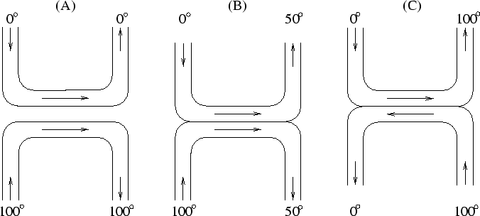
First consider a conventional, physical heat exchanger. See Figure 1 (C). There are two touching water pipes with opposite flow direction. Cold water enters the first pipe. Hot water enters the second pipe. But hot water exits the first pipe, and cold water exits the second pipe! At any given point where both pipes touch, their temperatures are the same (provided the water speed is low enough to allow for sufficient temperature exchange). Entirely local interaction can lead to a complete reversal of global, macroscopic properties such as temperature. Physical heat exchangers are common in technical applications (e.g., nuclear power plants) and animals, e.g., rodents (Geoff Hinton, personal communication, 1994).

Figure 1: (A) shows two water pipes that don't touch. Cold water enters and exits the first pipe. Hot water enters and exits the second pipe. (B) shows two touching water pipes with equal flow direction. Cold water enters the first pipe. Hot water enters the second pipe. Lukewarm water exits both. (C) shows two touching water pipes with opposite flow direction (a heat exchanger). Cold water enters the first pipe to become hot water. Hot water enters the second pipe to become cold water.

Basic idea. In analogy to the physical heat exchanger, I build a ``Neural Heat Exchanger''. There are two multi-layer feedforward networks with opposite flow direction. They correspond to the pipes. Both nets have the same number of layers. They are aligned such that each net's input layer is ``next'' to the other net's output layer, and each hidden layer in the first net is ``next'' to exactly one hidden layer in the other net. Input patterns enter the first net and are propagated ``up''. Desired outputs (targets) enter the ``opposite'' net and are propagated ``down''. Using the local, simple delta rule, each layer in each net tries to be similar (in information content) to the preceding layer and to the corresponding layer in the other net. The input entering the first net slowly ``heats up'' to become the target. The target entering the opposite net slowly ``cools down'' to become the input. No global control mechanism is required. See Figure 2 and details below.

Figure: The Neural Heat Exchanger requires two multi-layer feedforward nets with opposite flow direction. Each net's input layer is next to the other net's output layer. Each hidden layer in the upper net is next to exactly one hidden layer in the lower net. Input patterns enter the upper net and are propagated to the right. Desired outputs (targets) enter the lower net and are propagated to the left. Each layer in each net tries to be similar to the preceding layer and to the corresponding layer in the other net. For example, consider the black unit: two dotted lines connect the black unit to those two units it tries to match using the simple delta rule. Inputs entering the upper net slowly ``heat up'' to become like the targets. Targets entering the lower net slowly ``cool down'' to become like the inputs. No global control mechanism is required.

Architecture. See Figure 2. The first pipe corresponds to a feedforward network $F$ with n layers $F_1$, $F_2$, ..., $F_n$. Each unit in $F_i$ has directed connections to each unit in $F_{i+1}$, $i \in \{1, 2, \ldots, n-1 \}$. The second pipe corresponds to a feedforward network $B$ with n layers $B_1$, $B_2$, ..., $B_n$. Each unit in $B_{i+1}$ has directed connections to each unit in $B_i$, $i \in \{1, 2, \ldots, n-1 \}$. For simplicity, let all layers have m units. The $k$-th unit in $F_i$ is denoted $F_i^k$. The $k$-th unit in $B_i$ is denoted $B_i^k$. The randomly initialized weight on the connection from some unit $l$ to some unit $k$ is denoted $w_{kl}$.

Dynamics (example). See Figure 2. Input patterns enter $F$ at $F_1$. Output patterns exit $F$ at $F_n$. The goal is to make the output patterns like the targets. $B$'s flow direction is opposite to $F$'s. Targets (desired outputs) enter $B$ at $B_n$. Output patterns exit $B$ at $B_1$. The goal is to make the output patterns like $F$'s inputs. Input units are those in $F_1$ and $B_n$. At any given discrete time step, their activations are set by the environment, according to the current task. Furthermore, at any given time, each noninput unit $i$ updates its variable activation $o_i$ (initialized with 0.0) as follows: with probability $f(\sum_k w_{ik} o_k)$, set $o_i \leftarrow 1.0$; with probability $1 - f(\sum_k w_{ik} o_k)$, set $o_i \leftarrow 0.0$; where $f(x) = \frac{1}{1 + e^{-x}}$, for instance.

Learning. At any given discrete time step, using the simple delta rule (no backprop), weights are adjusted such that each noninput unit $F_i^k$ reduces its current (expected) distance to the corresponding unit $B_i^k$. Symmetrically: each noninput unit $B_i^k$ reduces its current distance to the corresponding unit $F_i^k$. Why? Because each layer should be similar to (``have the same temperature as'') the corresponding layer in the net with opposite flow direction.

Furthermore, at any given time step, using the simple delta rule (no backprop), weights are adjusted such that each noninput unit $F_i^k$ reduces its distance to unit $F^k_{i-1}$. Symmetrically: each noninput unit $B_i^k$ reduces its distance to $B^k_{i+1}$. Why? Because this tends to make successive units similar -- just like neighboring parts of a physical heat exchanger have similar temperature. The target entering $B$ slowly ``cools down'' to become the input. Likewise, the input entering $F$ slowly ``heats up'' to become the target.

Clearly, each weight gets error signals from two different local minimization processes. Simply add them up to change the weights.

Variants. The discussion above focused on the case where each layer has the same number of units. This makes it particularly convenient to define what it means for one layer to be similar to the preceding one: each unit's activation simply has to be similar to the one of the unit at the same position in the previous layer. Varying numbers of units per layer require us to refine our notion of layer similarity. For instance, layer similarity can be defined by measuring mutual information between successive layers. Non-probabilistic variants of the Neural Heat Exchanger may sometimes be appropriate as well.

Experiments. Three ETHZ undergrad students, Alberto Salerno, Thomas Fasciania, and Giorgio Pazmandi, recently reimplemented the Neural Heat Exchanger. They report that it was able to solve XOR more quickly than backprop. For larger scale parity problems, however, their system did not work as well as backprop. Sepp Hochreiter (personal communication) also implemented variants of the Neural Heat Exchanger. He learned simple functions such as AND with 5 and more hidden layers. He reports that the system prefers local coding in deep hidden layers. He also successfully tried variants where each layer has different numbers of units, and where either local auto-association or mutual information is used to define layer similarity. Unfortunately, however, at the moment of this writing, there has not yet been a detailed experimental study of the Neural Heat Exchanger. My own, very limited 1990 toy experiments also do not qualify as a systematic analysis. Much remains to be done.

Relation to recent work. According to Peter Dayan (personal communication, 1994), the Neural Heat Exchanger is essentially a supervised variant of the recent Helmholtz Machine [3,2]. Or, depending on the point of view, the Helmholtz Machine is an unsupervised variant of the Neural Heat Exchanger.

According to Peter Dayan and Geoff Hinton [1], a trouble with the Neural Heat Exchanger is that in non-deterministic domains, there is no reason why $B$'s output should match $F$'s input. Dayan and Hinton's algorithm overcomes this problem by using completely separate learning phases for top-down and bottom-up weights. This, however, makes their algorithm non-local in time: a global mechanism is required to separate the learning phases.

An alternative way to overcome the problem above may be to force part of $F$'s output to reconstruct a unique representation of $F$'s input, and to feed this representation also into $B$, together with the target.