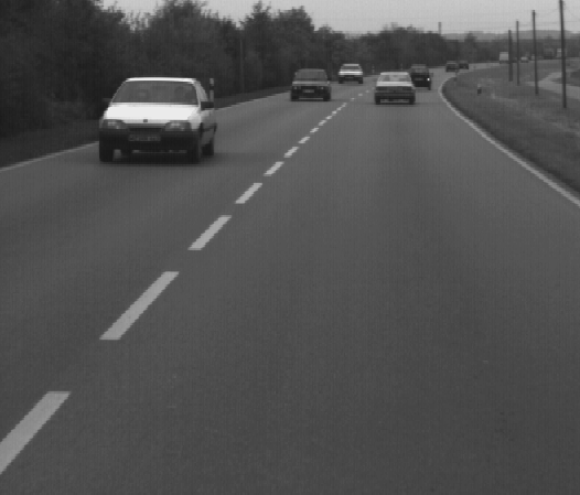
We apply PM
to static black and white images of driving cars (see Figure 2).
Each image is divided into
![]() square pixels.
Each pixel can take on 16 different grey levels represented
as integers scaled around zero.
square pixels.
Each pixel can take on 16 different grey levels represented
as integers scaled around zero.
Input generation. There is a circular ``input area''. Its diameter is 64 pixel widths. There are 32 code units. For each code unit, there is a ``bias input unit'' with constant activation 1.0, and a circular receptive field of 81 evenly distributed additional input units. The diameter of each receptive field is 20 pixel widths. Receptive fields partly overlap. The positions of code units and receptive fields relative to the input area are fixed. See Figure 3. The rotation of the input area is chosen randomly. Its position is chosen randomly within the boundaries of the image. The activation of an input unit is the average grey level value of the closest pixel and the four adjacent pixels (see Figure 4).
Learning: heuristic simplifications.
To achieve extreme computational simplicity
(and also biological plausibility),
we simplify the general method from section 2.
Heuristic simplifications are: (1) No error signals are
propagated through the predictor input units down into the code network.
(2) We focus on semilinear networks as opposed to general nonlinear ones
(no hidden units within predictors and code generating net - see Figure 1).
(3) Predictors and code units learn simultaneously
(also, each code unit sees only part of the total input).
These simplifications make the method local in both
space and time --
to change the weight of any predictor connection,
we can use the simple delta rule, which needs to
know only the current activations of the two connected units,
and the current activation of the unit to be predicted:
in response to input pattern
![]() , each weight
, each weight ![]() of predictor
of predictor ![]() changes according to
changes according to
|
figure=receptivefields.eps,width=
|
|
figure=activations.eps,width=
|
 |
|
figure=weights.eps,width=
|
|
figure=rotations.eps,width=
|
 |
Measuring information throughput.
Unsupervised learning is occasionally switched off.
Then the number ![]() of pairwise different output patterns
in response to 5000 randomly generated input patterns is determined
(the activation of each output unit is taken to be
0 if below 0.05, 1 if above 0.95,
and 0.5 otherwise).
The success rate is defined by
of pairwise different output patterns
in response to 5000 randomly generated input patterns is determined
(the activation of each output unit is taken to be
0 if below 0.05, 1 if above 0.95,
and 0.5 otherwise).
The success rate is defined by
![]() .
Clearly, a success rate
close to 1.0 implies high information throughput.
.
Clearly, a success rate
close to 1.0 implies high information throughput.
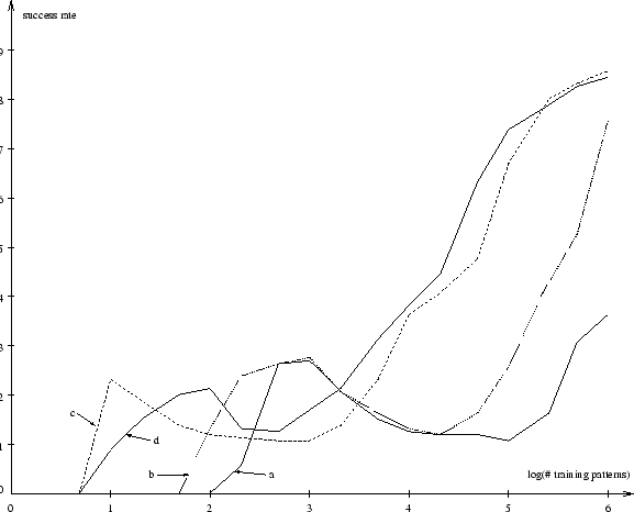
Results.
Figure 5 plots success rate against number of training pattern
presentations.
Results are shown for various pairs of predictor learning rates
![]() and code unit learning rates
and code unit learning rates ![]() .
For instance, with
.
For instance, with ![]() close to 1.0
and
close to 1.0
and ![]() being one or two orders of magnitude smaller,
high success rates are obtained.
Although the learning rates do have an influence on learning speed,
the basic shapes of the learning curves are similar.
being one or two orders of magnitude smaller,
high success rates are obtained.
Although the learning rates do have an influence on learning speed,
the basic shapes of the learning curves are similar.
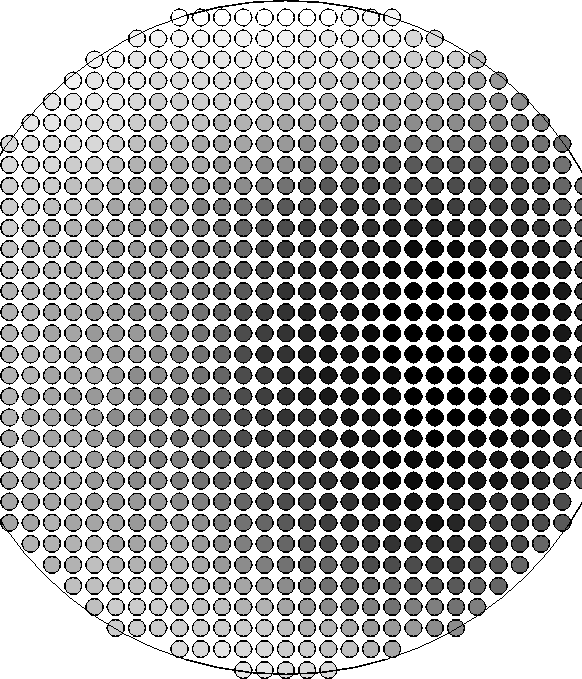
Edge detectors. With the set-up described above, to maximize information throughput, the system tends to create orientation sensitive edge detectors in an unsupervised manner. Weights corresponding to a typical receptive field (after 5000 pattern presentations) are shown in Figure 6. The connections are divided into two groups, one with inhibitory connections, the other one with excitatory connections. Both groups are separated by a ``fuzzy'' axis through the center of the receptive field. Its rotation angle determines the alignment of the edge provoking maximal response. In general, receptive fields of different code units exhibit different rotation angles. See Figure 7. Obviously, to represent the inputs in an informative but compact, efficient, redundancy-poor way, the creation of feature detectors specializing on certain rotated edges proves useful.
It is noticeable that in Figure 6 there appears to be a smooth gradient of weight strengths from strongly positive to strongly negative as one moves perpendicular to the positive/negative border. This is different from, e.g., MacKay and Miller (1990), where all weights tend to zero at the edge of the receptive field. At the moment, we don't have a good explanation for this effect.
On-center-off-surround / Off-center-on-surround. The nature of the receptive fields partly depends on receptive field size and degree of overlap. For instance, with nearly 200 input units per field and a more symmetric arrangement of receptive field centers (essentially, on the circular boundary of each field there are 6 other field centers), the system tends to generate another well-known kind of feature detector: the weight patterns become either on-center-off-surround-like or off-center-on-surround-like structures. See Figure 8 for an example.