In the comparatively simple case considered here,
the controller ![]() is a standard back-propagation network.
There are discrete time steps.
Each fovea trajectory involves
is a standard back-propagation network.
There are discrete time steps.
Each fovea trajectory involves ![]() discrete time steps 1 ...
discrete time steps 1 ... ![]() .
At time step
.
At time step ![]() of trajectory
of trajectory ![]() ,
, ![]() 's input is
the real-valued vector
's input is
the real-valued vector
![]() which is determined by sensory perceptions from
the artificial `fovea'.
which is determined by sensory perceptions from
the artificial `fovea'.
![]() 's output at time step
's output at time step ![]() of
trajectory
of
trajectory ![]() is the vector
is the vector
![]() .
At each time step
.
At each time step ![]() motoric actions like
`move fovea left', `rotate fovea' are based
on
motoric actions like
`move fovea left', `rotate fovea' are based
on ![]() . The actions cause a new input
. The actions cause a new input ![]() .
The final desired input
.
The final desired input ![]() of the trajectory
of the trajectory
![]() is a
predefined activation pattern
corresponding to the target to be found in
a static visual scene.
The task is to sequentially
generate fovea trajectories such that for each trajectory
is a
predefined activation pattern
corresponding to the target to be found in
a static visual scene.
The task is to sequentially
generate fovea trajectories such that for each trajectory ![]()
![]() matches
matches ![]() .
The final input error
.
The final input error ![]() at
the end of trajectory
at
the end of trajectory ![]() (externally interrupted
at time step
(externally interrupted
at time step ![]() ) is
) is
Thus ![]() is determined by the differences between the
desired final inputs and the actual final inputs.
is determined by the differences between the
desired final inputs and the actual final inputs.
In order to allow credit assignment to past output actions
of the control network, we first train the
model network ![]() (another standard back-propagation network)
to emulate the visible environmental
dynamics. This is done by training
(another standard back-propagation network)
to emulate the visible environmental
dynamics. This is done by training ![]() at
a given time to
predict
at
a given time to
predict ![]() 's next input, given
the previous input and output of
's next input, given
the previous input and output of ![]() .
The following discussion refers to the case where both
.
The following discussion refers to the case where both ![]() and
and
![]() learn in parallel. In some of the experiments below we use
two separate training phases for
learn in parallel. In some of the experiments below we use
two separate training phases for ![]() and
and ![]() . However, the
modifications are straight-forward and mainly notational.
. However, the
modifications are straight-forward and mainly notational.
![]() 's input vector at time
's input vector at time ![]() of trajectory
of trajectory ![]() is the
concatenation of
is the
concatenation of ![]() and
and ![]() .
.
![]() 's real-valued output vector at time
's real-valued output vector at time ![]() of trajectory
of trajectory ![]() is
is ![]() ,
where
,
where
![]() . (Here
. (Here ![]() is the
dimension of
is the
dimension of ![]() ,
, ![]() has as many
output units as there are input units for
has as many
output units as there are input units for ![]() .)
.) ![]() is
is ![]() 's
prediction of
's
prediction of ![]() .
The error of
.
The error of ![]() 's prediction at time
's prediction at time ![]() of trajectory
of trajectory ![]() is
is
![]() 's goal is to minimize
's goal is to minimize
![]() , which is done
by conventional back-propagation
[17][7][4][9]:
, which is done
by conventional back-propagation
[17][7][4][9]:
![]() 's training phase is more complex than
's training phase is more complex than ![]() 's.
It is assumed that
's.
It is assumed that
![]() is a differentiable function of
is a differentiable function of ![]() ,
where
,
where ![]() is
is ![]() 's weight vector. To approximate
's weight vector. To approximate
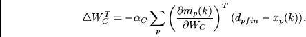
Here
![]() is
is ![]() 's
increment caused by the back-propagation procedure,
and
's
increment caused by the back-propagation procedure,
and ![]() is the learning rate of the controller.
Note that
the differences between target inputs and actual final inputs
at the end of each trajectory
are used for computing error signals for the controller. We
do not use
the differences
between desired final inputs and predicted final inputs.
is the learning rate of the controller.
Note that
the differences between target inputs and actual final inputs
at the end of each trajectory
are used for computing error signals for the controller. We
do not use
the differences
between desired final inputs and predicted final inputs.
To apply the `unfolding in time' algorithm
[9][18]
to the recurrent combination of ![]() and
and ![]() , do the
following:
, do the
following:
For all trajectories ![]() :
:
1. During the activation spreading phase of ![]() ,
for each time step
,
for each time step ![]() of
of ![]() create a copy of
create a copy of ![]() (called
(called ![]() ) and a copy of
) and a copy of ![]() (called
(called ![]() ).
).
2. Construct a large `unfolded' feed-forward
back-propagation network consisting of ![]() sub-modules by doing the following:
sub-modules by doing the following:
2.a) For ![]() replace each input unit
replace each input unit ![]() of
of ![]() by the unit in
by the unit in
![]() which predicted
which predicted ![]() 's activation.
's activation.
2.b) For ![]() :
Replace each input unit of
:
Replace each input unit of ![]() whose activation was provided
by an output unit
whose activation was provided
by an output unit ![]() of
of ![]() by
by ![]() .
.
3. Propagate the difference
![]() back
through the entire `unfolded' network constructed in step 2.
Change each weight of
back
through the entire `unfolded' network constructed in step 2.
Change each weight of ![]() in proportion to the sum of the
partial derivatives
computed for the corresponding
in proportion to the sum of the
partial derivatives
computed for the corresponding ![]() connection copies in the unfolded
network. Do not change the weights of
connection copies in the unfolded
network. Do not change the weights of ![]() .
.
Since the weights remain constant during the activation
spreading phase of one trajectory, the practical algorithm used in
the experiments
does not really create copies of the weights.
It is more efficient to introduce one additional variable
for each controller weight: This variable is used for
accumulating the corresponding
sum of weight changes.
During trajectory execution, it is convenient to push
the time-varying activations of
the units in ![]() and
and ![]() on
stacks of activations, one for each unit.
During the back-propagation phase these
activations can be successively popped off for the
computation of error signals.
on
stacks of activations, one for each unit.
During the back-propagation phase these
activations can be successively popped off for the
computation of error signals.