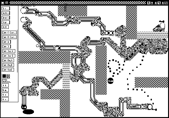
Environment.
Figure 1
![]() (click here or see below) shows
a partially observable environment (POE)
with
(click here or see below) shows
a partially observable environment (POE)
with
![]() pixels.
This POE has many more states and
obstacles than most reported in the POE literature --
for instance, Littman et al.'s largest problem
[#!Littman:94!#]
involves less than 1000 states.
There are two SMP/SSA-based
agents A and B. Each has circular shape and a diameter of
30 pixels. At a given time, each is rotated in
one of eight different directions.
State space size exceeds 1013 by far,
not even taking into account
internal states (IP values) of the agents.
pixels.
This POE has many more states and
obstacles than most reported in the POE literature --
for instance, Littman et al.'s largest problem
[#!Littman:94!#]
involves less than 1000 states.
There are two SMP/SSA-based
agents A and B. Each has circular shape and a diameter of
30 pixels. At a given time, each is rotated in
one of eight different directions.
State space size exceeds 1013 by far,
not even taking into account
internal states (IP values) of the agents.
There are also two keys, key A (only useful for agent A) and
key B (only for agent B), and two locked doors,
door A and door B, the only entries to room A and room B, respectively.
Door A (B) can be opened only with key A (B).
At the beginning of each ``trial'',
both agents are randomly rotated and placed
near the northwest corner, all doors are closed,
key A is placed in the southeast corner,
and key B is placed in room A (see Figure 1 ![]() ).
).
Task. The goal of each agent is to reach the goal in room B. This requires cooperation: (1) agent A must first find and take key A (by touching it); (2) then agent A must go to door A and open it (by touching it) for agent B; (3) then agent B must enter through door A, find and take key B; (4) then agent B must go to door B to open it (to free the way to the goal); (5) then at least one of the agents must reach the goal position. For each turn or move there is a small penalty (immediate reward -0.0001).
Positive reward is generated only if one of the agents touches the goal. This agent's reward is 5.0; the other's is 3.0 (for its cooperation -- note that asymmetric reward introduces competition). Only then a new trial starts. There is no maximal trial length, and the agents have no a priori concept of a trial. Time is not reset when a new trial starts.
Instruction set.
Both agents share the same design. Each is equipped
with limited ``active'' sight: by executing certain instructions,
it can sense obstacles, its own key,
the corresponding door, or the goal,
within up to 10 ``steps'' in front of it.
The step size is 5 pixel widths.
The agent can also move forward, turn around, turn relative
to its key or its door or the goal.
Directions are represented as integers in
![]() :
0 for north, 1 for northeast, 2 for east, etc.
Each agent has m=52 program cells, and
nops=13 instructions (including
JumpHome/PLA/evaluation instructions
B0, B1, B2 from section 3):
:
0 for north, 1 for northeast, 2 for east, etc.
Each agent has m=52 program cells, and
nops=13 instructions (including
JumpHome/PLA/evaluation instructions
B0, B1, B2 from section 3):
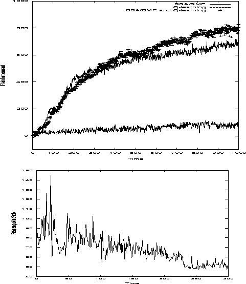
Results without learning. If we switch off SMP's self-modifying capabilities (IncProb has no effect), then the average trial length is 330,000 basic cycles (random behavior).
Results with Q-Learning.
Q-learning assumes that the environment is fully observable;
otherwise it is not guaranteed to work. Still, some
authors occasionally apply Q-learning variants to
partially observable environments, sometimes even successfully
[#!Crites:96!#].
To test whether our problem is indeed too difficult
for Q-learning, we tried to solve it using various
![]() Q-variants [#!Lin:93!#].
We first used primitive actions and
perceptions similar to SMP's instructions.
There are 33 possible Q-actions. The first 32 are
``turn to one of the 8 different directions relative
to the agent's key/door/current direction/goal,
and move 3 steps forward''. The 33rd action allows for
turning without moving: ``turn 45 degrees to the right''.
These actions are more powerful than SMP's instructions
(most combine two actions similar to SMP's into one).
There are 2*5 = 10 different inputs telling the
agent whether it has/hasn't got its key, and whether
the closest object (obstacle, key, door, or goal)
part of which is either 10, 20, 30, 40, or 50 pixels
in front of the agent is
obstacle/key/door/goal/non-existent.
All of this corresponds to 10 rows and 33 columns in the Q-tables.
Q-learning's parameters are
Q-variants [#!Lin:93!#].
We first used primitive actions and
perceptions similar to SMP's instructions.
There are 33 possible Q-actions. The first 32 are
``turn to one of the 8 different directions relative
to the agent's key/door/current direction/goal,
and move 3 steps forward''. The 33rd action allows for
turning without moving: ``turn 45 degrees to the right''.
These actions are more powerful than SMP's instructions
(most combine two actions similar to SMP's into one).
There are 2*5 = 10 different inputs telling the
agent whether it has/hasn't got its key, and whether
the closest object (obstacle, key, door, or goal)
part of which is either 10, 20, 30, 40, or 50 pixels
in front of the agent is
obstacle/key/door/goal/non-existent.
All of this corresponds to 10 rows and 33 columns in the Q-tables.
Q-learning's parameters are
![]() ,
,
![]() ,
and learning rate 0.001
(these worked well for smaller problems Q-learning was able
to solve). For each executed action there is an immediate
small penalty of -0.0001, to let Q-learning favor
shortest paths.
,
and learning rate 0.001
(these worked well for smaller problems Q-learning was able
to solve). For each executed action there is an immediate
small penalty of -0.0001, to let Q-learning favor
shortest paths.
This Q-learning variant, however, utterly failed to achieve
significant performance improvement.
We then tried to make the problem
easier (more observable) by
extending the agent's sensing capabilities.
Now each possible input tells the agent uniquely whether
it has/hasn't got the key,
and whether the closest object (obstacle or key or door or goal)
part of which is either 10, 20, 30, 40, or 50 pixels away
in front of/45 degrees to the right of/45 degrees to the left of the agent is
obstacle/key/door/goal/non-existent,
and if existing, whether it is 10/20/30/40/50 pixels away.
All this can be efficiently coded by
![]() different inputs corresponding to 18522 different
rows in the Q-tables (with a total of 611226 entries).
This worked indeed a bit better than the simpler Q-variant.
Still, we were not able to make Q-learning achieve very
significant performance improvement --
see Figure 2
different inputs corresponding to 18522 different
rows in the Q-tables (with a total of 611226 entries).
This worked indeed a bit better than the simpler Q-variant.
Still, we were not able to make Q-learning achieve very
significant performance improvement --
see Figure 2 ![]() .
.
Results with SMP/SSA.
After 109 basic cycles
(ca. 130,000 trials), average trial length was
5500 basic cycles
(mean of 4 simulations).
This is about 60 times faster than the
initial random behavior,
and roughly
![]() to
to
![]() of the optimal speed
estimated by hand-crafting a solution
(due to the POE setting and the
random trial initializations
it is very hard to calculate optimal average speed).
Typical results are shown in Figures 2
of the optimal speed
estimated by hand-crafting a solution
(due to the POE setting and the
random trial initializations
it is very hard to calculate optimal average speed).
Typical results are shown in Figures 2 ![]() and 3
and 3 ![]() .
.
Q-learning as an instruction for SMP.
Q-learning is not designed for POEs. This
does not mean, however,
that Q-learning cannot be plugged into
SMP/SSA as a sometimes useful instruction.
To examine this issue, we add
![]() Q-learning [#!Lin:93!#].
to the instruction set of both agents' SMPs:
Q-learning [#!Lin:93!#].
to the instruction set of both agents' SMPs:
 |
 |
Observations.
Final stack sizes never exceeded 250,
corresponding to about 250 surviving SMP-modifications.
This is just a small fraction of the about
![]() self-modifications executed during each agent's life.
It is interesting to observe how the agents use self-modifications
to adapt self-modification frequency itself.
Towards death they learn
that there is not as much to learn any more, and
decrease this frequency (self-generated annealing schedule, see
Figure 3
self-modifications executed during each agent's life.
It is interesting to observe how the agents use self-modifications
to adapt self-modification frequency itself.
Towards death they learn
that there is not as much to learn any more, and
decrease this frequency (self-generated annealing schedule, see
Figure 3 ![]() ). It should be mentioned
that the adaptive distribution of self-modifications
is highly non-uniform. It often temporarily focuses on
currently ``promising'' individual SMP-components.
In other words, the probabilistic self-modifying
learning algorithm itself occasionally changes based on
previous experience.
). It should be mentioned
that the adaptive distribution of self-modifications
is highly non-uniform. It often temporarily focuses on
currently ``promising'' individual SMP-components.
In other words, the probabilistic self-modifying
learning algorithm itself occasionally changes based on
previous experience.