Assume that the alphabet contains
![]() possible characters
possible characters
![]() .
The (local) representation of
.
The (local) representation of ![]() is a binary
is a binary ![]() -dimensional
vector
-dimensional
vector ![]() with exactly one non-zero component (at the
with exactly one non-zero component (at the ![]() -th position).
-th position).
![]() has
has ![]() input units and
input units and ![]() output units.
output units.
![]() is called the ``time-window'' size.
We insert
is called the ``time-window'' size.
We insert ![]() default characters
default characters ![]() at the beginning of each file.
The representation of the
default character,
at the beginning of each file.
The representation of the
default character, ![]() , is the
, is the ![]() -dimensional zero-vector.
The
-dimensional zero-vector.
The ![]() -th character of file
-th character of file ![]() (starting
from the first default character) is called
(starting
from the first default character) is called ![]() .
.
For all ![]() and all possible
and all possible ![]() ,
,
![]() receives as an input
receives as an input
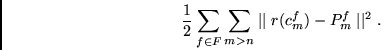 |
(1) |
| (2) |
| (3) |
For instance, assume that a given
``context string'' of size ![]() is followed by a certain character
in one third of all training exemplars
involving this string.
Then, given the context,
the predictor's corresponding output unit
will tend to predict a value of 0.3333.
is followed by a certain character
in one third of all training exemplars
involving this string.
Then, given the context,
the predictor's corresponding output unit
will tend to predict a value of 0.3333.
In practical applications, the
![]() will not always sum up to 1.
To obtain outputs satisfying the properties of
a proper probability distribution,
we normalize by defining
will not always sum up to 1.
To obtain outputs satisfying the properties of
a proper probability distribution,
we normalize by defining
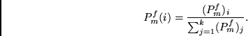 |
(4) |