Reward/Goal. Occasionally ![]() provides real-valued reward.
provides real-valued reward. ![]() is
the cumulative reward obtained between time 0 and time
is
the cumulative reward obtained between time 0 and time ![]() , where
, where
![]() . At time
. At time ![]() the learner's goal is to accelerate long-term
reward intake: it wants to let
the learner's goal is to accelerate long-term
reward intake: it wants to let
![]() exceed the
current average reward intake.
To compute the ``current average reward intake'' a previous point
exceed the
current average reward intake.
To compute the ``current average reward intake'' a previous point
![]() to compute
to compute
![]() is required.
How to specify
is required.
How to specify ![]() in a general yet reasonable way? For instance,
if life consists of many successive ``trials'' with non-deterministic
outcome, how many trials must we look back in time? This question will
be addressed by the success-story algorithm (SSA) below.
in a general yet reasonable way? For instance,
if life consists of many successive ``trials'' with non-deterministic
outcome, how many trials must we look back in time? This question will
be addressed by the success-story algorithm (SSA) below.
Initialization. At time ![]() (system birth), we initialize the
learner's variable internal state
(system birth), we initialize the
learner's variable internal state ![]() , a vector of variable, binary
or real-valued components. Environmental inputs may be represented by
certain components of
, a vector of variable, binary
or real-valued components. Environmental inputs may be represented by
certain components of ![]() . We also initialize the vector-valued
policy
. We also initialize the vector-valued
policy ![]() .
. ![]() 's
's ![]() -th variable component is denoted
-th variable component is denoted ![]() .
There is a set of possible actions to be selected and executed according
to current
.
There is a set of possible actions to be selected and executed according
to current ![]() and
and ![]() . For now, there is no need to specify
. For now, there is no need to specify
![]() -- this will be done in the experimental sections (typically,
-- this will be done in the experimental sections (typically,
![]() will be a conditional probability distribution on the possible
next actions, given current
will be a conditional probability distribution on the possible
next actions, given current ![]() ). We introduce an initially empty
stack
). We introduce an initially empty
stack ![]() that allows for stack entries with varying sizes, and
the conventional push and pop operations.
that allows for stack entries with varying sizes, and
the conventional push and pop operations.
Basic cycle.
Between time 0 (system birth) and time ![]() (system death)
the following basic cycle is repeated over and over again:
(system death)
the following basic cycle is repeated over and over again:
IF there is no ``tag'' (a pair of time and cumulative
reward until then) stored somewhere in ![]() ,
,
THEN push the tag (![]() ,
, ![]() ) onto
) onto ![]() , and go to 3
(this ends the current SSA call).
, and go to 3
(this ends the current SSA call).
ELSE denote the topmost tag in ![]() by (
by (![]() ,
, ![]() ).
Denote the one below by (
).
Denote the one below by (![]() ,
, ![]() ) (if there is not any tag below,
set variable
) (if there is not any tag below,
set variable ![]() -- recall
-- recall
![]() ).
).
ELSE pop off all stack entries above the one for tag (![]() ,
,
![]() ) (these entries will be former policy components saved during
earlier executions of step 3), and use them to restore
) (these entries will be former policy components saved during
earlier executions of step 3), and use them to restore ![]() as it
was be before time
as it
was be before time ![]() . Then also pop off the tag (
. Then also pop off the tag (![]() ,
, ![]() ).
Go to SSA.1.
).
Go to SSA.1.
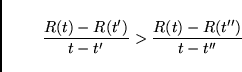
SSA ensures life-time success stories.
At a given time in the
learner's life, define the set of currently valid times as those
previous times still stored in tags somewhere in ![]() . If this set
is not empty right before tag
. If this set
is not empty right before tag ![]() is pushed in step SSA.2 of
the basic cycle, then let
is pushed in step SSA.2 of
the basic cycle, then let
![]() denote
the
denote
the ![]() -th valid time, counted from the bottom of
-th valid time, counted from the bottom of ![]() . It is easy
to show (Schmidhuber, 1994, 1996) that the current SSA call will have
enforced the following ``success-story criterion'' SSC (
. It is easy
to show (Schmidhuber, 1994, 1996) that the current SSA call will have
enforced the following ``success-story criterion'' SSC (![]() is the
is the ![]() in the most recent step SSA.2):
in the most recent step SSA.2):
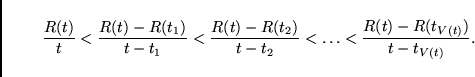 |
(1) |
SSA's generalization assumption.
Since life is one-way (time is never reset), during each SSA call the
system has to generalize from a single experience concerning the
usefulness of any previous policy modification:
the average reward per time since then.
At the end of each SSA call,
until the beginning of the next one, the only temporary generalization
assumption for inductive inference is: ![]() -modifications that survived
all previous SSA calls will remain useful.
In absence of empirical
evidence to the contrary, each still valid sequence of
-modifications that survived
all previous SSA calls will remain useful.
In absence of empirical
evidence to the contrary, each still valid sequence of ![]() -modifications
is assumed to have successfully set the stage for later ones.
What has appeared useful so far will get another chance to justify itself.
-modifications
is assumed to have successfully set the stage for later ones.
What has appeared useful so far will get another chance to justify itself.
When will SSC be satisfiable in a non-trivial way? In irregular
and random environments there is no way of justifying permanent policy
modifications by SSC. Also, a trivial way of satisfying SSC is to
never make a modification. Let us assume, however, that ![]() ,
, ![]() , and action set
, and action set ![]() (representing the system's initial bias)
do indeed allow for
(representing the system's initial bias)
do indeed allow for ![]() -modifications triggering long-term reward
accelerations. This is an instruction set-dependent assumption much
weaker than the typical Markovian assumptions made in previous RL
work, e.g., [#!Kumar:86!#,#!Sutton:88!#,#!WatkinsDayan:92!#,#!Williams:92!#].
Now, if we prevent all instruction probabilities from vanishing (see
concrete implementations in sections 3/4), then the system will execute
-modifications triggering long-term reward
accelerations. This is an instruction set-dependent assumption much
weaker than the typical Markovian assumptions made in previous RL
work, e.g., [#!Kumar:86!#,#!Sutton:88!#,#!WatkinsDayan:92!#,#!Williams:92!#].
Now, if we prevent all instruction probabilities from vanishing (see
concrete implementations in sections 3/4), then the system will execute
![]() -modifications occasionally, and keep those consistent with SSC.
In this sense, it cannot help getting better. Essentially, the system
keeps generating and undoing policy modifications until it discovers
some that indeed fit its generalization assumption.
-modifications occasionally, and keep those consistent with SSC.
In this sense, it cannot help getting better. Essentially, the system
keeps generating and undoing policy modifications until it discovers
some that indeed fit its generalization assumption.
Greediness? SSA's strategy appears greedy. It always keeps the policy that was observed to outperform all previous policies in terms of long-term reward/time ratios. To deal with unknown reward delays, however, the degree of greediness is learnable -- SSA calls may be triggered or delayed according to the modifiable policy itself.
Actions can be almost anything. For instance, an action executed in step 3 may be a neural net algorithm. Or it may be a Bayesian analysis of previous events. While this analysis is running, time is running, too. Thus, the complexity of the Bayesian approach is automatically taken into account. In section 3 we will actually plug in an adaptive Levin search extension. Similarly, actions may be calls of a Q-learning variant -- see experiments in [#!Schmidhuber:96meta!#]. Plugging Q into SSA makes sense in situations where Q by itself is questionable because the environment might not satisfy the preconditions that would make Q sound. SSA will ensure, however, that at least each policy change in the history of all still valid policy changes will represent a long-term improvement, even in non-Markovian settings.
Limitations. (1) In general environments neither SSA nor any other scheme is guaranteed to continually increase reward intake per fixed time interval, or to find the policy that will lead to maximal cumulative reward. (2) No reasonable statements can be made about improvement speed which indeed highly depends on the nature of the environment and the choice of initial, ``primitive'' actions (including learning algorithms) to be combined according to the policy. This lack of quantitative convergence results is shared by many other, less general RL schemes though (recall that Q-learning is not guaranteed to converge in finite time).
Outline of remainder. Most of our paper will be about plugging various policy-modifying algorithms into the basic cycle. Despite possible implementation-specific complexities the overall concept is very simple. Sections 3 and 4 will describe two concrete implementations. The first implementation's action set consists of a single but ``strong'' policy-modifying action (a call of a Levin search extension). The second implementation uses many different, less ``powerful'' actions. They resemble assembler-like instructions from which many different policies can be built (the system's modifiable learning strategy is able to modify itself). Experimental case studies will involve complex environments where standard RL algorithms fail. Section 5 will conclude.