FMS Overview. FMS is a general method for finding low complexity-networks with high generalization capability. FMS finds a large region in weight space such that each weight vector from that region has similar small error. Such regions are called ``flat minima''. In MDL terminology, few bits of information are required to pick a weight vector in a ``flat'' minimum (corresponding to a low complexity-network) -- the weights may be given with low precision. In contrast, weights in a ``sharp'' minimum require a high-precision specification. As a natural by-product of net complexity reduction, FMS automatically prunes weights and units, and reduces output sensitivity with respect to remaining weights and units. Previous FMS applications focused on supervised learning (Hochreiter and Schmidhuber 1995, 1997a): FMS led to better stock market prediction results than ``weight decay'' and ``optimal brain surgeon'' (Hassibi and Stork 1993). In this paper, however, we will use it for unsupervised coding only.
Architecture.
We use a 3-layer feedforward net.
Each layer is fully connected to the next.
Let ![]() denote
index sets for output, hidden, input units, respectively.
Let
denote
index sets for output, hidden, input units, respectively.
Let
![]() denote the number of elements in a set.
For
denote the number of elements in a set.
For
![]() , the activation
, the activation ![]() of unit
of unit ![]() is
is
![]() , where
, where
![]() is the net input of unit
is the net input of unit ![]() (
(![]() for
for ![]() and
and ![]() for
for ![]() ),
),
![]() denotes the
weight on the connection from unit
denotes the
weight on the connection from unit ![]() to unit
to unit ![]() ,
,
![]() denotes unit
denotes unit ![]() 's activation function,
and for
's activation function,
and for ![]() ,
, ![]() denotes the
denotes the ![]() -th
component of an input vector.
-th
component of an input vector.
![]() is the number of weights.
is the number of weights.
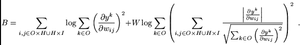
Algorithm.
FMS' objective function ![]() features an unconventional error term:
features an unconventional error term: