Task.
Figure 1
shows
a ![]() -maze
with a single start position (S) and a
single goal position (G). The maze has many more fields and
obstacles than mazes used by previous
authors working on POMDPs
(for instance, McCallum's maze has only 23 free fields
[McCallum, 1995]).
The goal is to find a program that makes an
agent move from S to G.
-maze
with a single start position (S) and a
single goal position (G). The maze has many more fields and
obstacles than mazes used by previous
authors working on POMDPs
(for instance, McCallum's maze has only 23 free fields
[McCallum, 1995]).
The goal is to find a program that makes an
agent move from S to G.
Instructions.
Programs can be
composed from 9 primitive instructions. These instructions
represent the initial bias provided by the programmer
(in what follows, superscripts will indicate instruction
numbers).
The first 8 instructions have the following syntax : REPEAT
step forward UNTIL condition 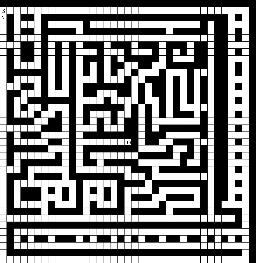 , THEN rotate towards direction
 ![]() .
.
Instruction 1 : = front is blocked, ![]() = left.
= left.
Instruction 2 : = front is blocked, ![]() = right.
= right.
Instruction 3 : = left field is free, ![]() = left.
= left.
Instruction 4 : = left field is free, ![]() = right.
= right.
Instruction 5 : = left field is free, ![]() = none.
= none.
Instruction 6 : = right field is free, ![]() = left.
= left.
Instruction 7 : = right field is free, ![]() = right.
= right.
Instruction 8 : = right field is free, ![]() = none.
= none.
Instruction 9 is: Jump(address, nr-times).
It has two parameters: nr-times
![]() , and
address
, and
address
![]() , where
, where ![]() is the highest address in the current program.
Jump uses an additional hidden variable nr-times-to-go which
is initially set to nr-times.
The semantics are:
If nr-times-to-go
is the highest address in the current program.
Jump uses an additional hidden variable nr-times-to-go which
is initially set to nr-times.
The semantics are:
If nr-times-to-go ![]() , continue execution at address address.
If
, continue execution at address address.
If ![]() nr-times-to-go
nr-times-to-go ![]() , decrement nr-times-to-go.
If nr-times-to-go
, decrement nr-times-to-go.
If nr-times-to-go ![]() , set nr-times-to-go to nr-times.
Note that nr-times
, set nr-times-to-go to nr-times.
Note that nr-times ![]() may cause an infinite loop.
The Jump instruction is essential for exploiting the possibility that
solutions may consist of repeatable action sequences and
``subprograms'' (thus having low algorithmic complexity).
LS' incrementally growing time limit automatically deals with
those programs that don't halt, by preventing them from consuming
too much time.
may cause an infinite loop.
The Jump instruction is essential for exploiting the possibility that
solutions may consist of repeatable action sequences and
``subprograms'' (thus having low algorithmic complexity).
LS' incrementally growing time limit automatically deals with
those programs that don't halt, by preventing them from consuming
too much time.
As mentioned in section 2,
the probability of a program is
the product of the probabilities
of its constituents.
To deal with probabilities
of the two Jump parameters,
we introduce two additional variable matrices,
![]() and
and ![]() .
For a program with
.
For a program with ![]() instructions,
to specify the conditional probability
instructions,
to specify the conditional probability ![]() of a
jump to address
of a
jump to address ![]() , given that the instruction
at address
, given that the instruction
at address ![]() is Jump
(
is Jump
(
![]() ,
,
![]() ),
we first normalize the entries
),
we first normalize the entries
![]() ,
,
![]() ,
...,
,
...,
![]() (this ensures that the relevant entries sum up to 1).
Provided the instruction at address
(this ensures that the relevant entries sum up to 1).
Provided the instruction at address ![]() is Jump,
for
is Jump,
for
![]() ,
,
![]() ,
, ![]() specifies the probability of the nr-times parameter
being set to
specifies the probability of the nr-times parameter
being set to ![]() .
Both
.
Both ![]() and
and ![]() are initialized uniformly
and are adapted by ALS just like
are initialized uniformly
and are adapted by ALS just like ![]() itself.
itself.
Restricted LS-variant. Note that the instructions above are not sufficient to build a universal programming language -- the experiments in this paper are confined to a restricted version of LS. From the instructions above, however, one can build programs for solving any maze in which it is not necessary to completely reverse the direction of movement (rotation by 180 degrees) in a corridor. Note that it is mainly the Jump instruction that allows for composing low-complexity solutions from ``subprograms'' (LS provides a sound way for dealing with infinite loops).
Rules. Before LS generates, runs and tests a new program, the agent is reset to its start position. Collisions with walls halt the program. A path generated by a program that makes the agent hit the goal is called a solution (the agent is not required to stop at the goal -- there are no explicit halt instructions).
Why is this a POMDP? Because the instructions above are not sufficient to tell the agent exactly where it is: at a given time, the agent can perceive only one of three highly ambiguous types of input (by executing the appropriate primitive): ``front is blocked or not'', ``the left field is free or not'', ``the right field is free or not'' (compare list of primitives). Some sort of memory is required to disambiguate apparently equal situations encountered on the way to the goal. Q-learning, for instance, is not guaranteed to solve POMDPs (e.g, [Watkins and Dayan, 1992]). Our agent, however, can use memory implicit in the state of the execution of its current program to disambiguate ambiguous situations.
Measuring time. The computational cost of a single Levin search call in between two Adapt calls is essentially the sum of the costs of all the programs it tests. To measure the cost of a single program, we simply count the total number of forward steps and rotations during program execution (this number is of the order of total computation time). Note that instructions often cost more than 1 step! To detect infinite loops, LS also measures the time consumed by Jump instructions (one time step per executed Jump). In a realistic application, however, the time consumed by a robot move would by far exceed the time consumed by a Jump instruction -- we omitted this (negligible) cost in the experimental results.
Comparison.
We compared LS to
three variants of Q-learning [Watkins and Dayan, 1992] and
random search.
Random search repeatedly and randomly selects and executes one of the
instructions (1-8) until the goal is hit (like with Levin search,
the agent is
reset to its start position whenever it hits the wall).
Since random search (unlike LS) does not have a
time limit for testing, it may not use the jump - this
is to prevent it from wandering into infinite loops.
The first Q-variant uses the same 8 instructions, but has the
advantage that it can distinguish all possible states
(952 possible inputs -- but this
actually makes the task much easier, because it is no POMDP any more).
The first Q-variant was just tested to see how much more
difficult the problem becomes in the POMDP setting.
The second
Q-variant can only observe whether the four surrounding fields are
blocked or not (16 possible inputs), and the third
Q-variant receives a unique representation of the five most recent
executed instructions as input (37449 possible inputs -- this
requires a gigantic Q-table!).
Actually,
after a few initial experiments with the second Q-variant,
we noticed that it could not use its input for preventing
collisions
(the agent always walks for a while and then rotates --
in front of a wall, every instruction will cause a collision).
To improve the second Q-variant's performance,
we appropriately altered the instructions: each
instruction consists of one of the 3 types of rotations followed
by one of the 3 types of forward walks
(thus the total number of instructions is 9 --
for the same reason as with random search,
the jump instruction cannot be used).
The parameters of the Q-learning
variants were first coarsely optimized on a number of smaller
mazes which they were able to solve.
We set ![]() , which means that in the first
phase (
, which means that in the first
phase (![]() = 1 in the LS procedure), a
program with probability 1 may execute
up to 200 steps before being stopped.
= 1 in the LS procedure), a
program with probability 1 may execute
up to 200 steps before being stopped.
Typical result.
In the easy, totally observable
case, Q-learning
took on average 694,933 steps (10 simulations were conducted)
to solve the maze from Figure 1.
However, as expected,
in the difficult, partially observable cases,
neither the two Q-learning variants
nor random search
were ever able to solve the maze within
1,000,000,000 steps (5 simulations were conducted).
In contrast, LS was indeed able to solve the POMDP:
LS required 97,395,311 steps
to find a program ![]() computing a 127-step shortest path to the goal in
Figure 1.
LS' low-complexity solution involves two nested loops:
computing a 127-step shortest path to the goal in
Figure 1.
LS' low-complexity solution involves two nested loops:
1) REPEAT step forward UNTIL left
field is free
2) Jump (1 , 3)
3) REPEAT step forward UNTIL left
field is free, rotate left
4) Jump (1 , 5)
Similar results were obtained with many other mazes having non-trivial solutions with low algorithmic complexity. Such experiments illustrate that smart search through program space can be beneficial in cases where the task appears complex but actually has low-complexity solutions. Since LS has a principled way of dealing with non-halting programs and time-limits (unlike, e.g., ``Genetic Programming''(GP)), LS may also be of interest for researchers working in GP and related fields (the first paper on using GP-like algorithms to evolve assembler-like computer programs was, to the best of our knowledge, [Dickmanns et al., 1987]).
ALS: single tasks versus multiple tasks. If we use the adaptive LS extension (ALS) for a single task as the one above (by repeatedly applying LS to the same problem and changing the underlying probability distribution in between successive calls according to section 3), then the probability matrix rapidly converges such that late LS calls find the solution almost immediately. This is not very interesting, however -- once the solution to a single problem is found (and there are no additional problems), there is no point in investing additional efforts into probability updates. ALS is more interesting in cases where there are multiple tasks, and where the solution to one task conveys some but not all information helpful for solving additional tasks. This is what the next section is about.