Next: Error path integral
Up: Exponential error decay
Previous: Exponential error decay
The results we are going to prove
hold regardless of the particular kind of cost function used (as long
as its continuous in the output) and
regardless of the particular algorithm which is employed to compute the gradient.
Here we shortly explain how gradients are computed by the standard
BPTT algorithm (e.g., [27], see also
crossreference Chapter 14 for more details) because its analytical
form is better suited to the forthcoming analyses.
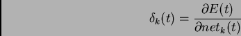
The error at time  is denoted by
  .
Considering only the error at time , output unit
.
Considering only the error at time , output unit  's error signal is
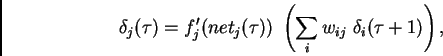
and some non-output unit  's backpropagated error signal
at time
's backpropagated error signal
at time  is
is
where
is unit  's current net input,
is the activation of
a non-input unit
with differentiable transfer function  ,
and
,
and  is the weight on the connection from unit to .
The corresponding contribution
to
is the weight on the connection from unit to .
The corresponding contribution
to  's total weight update is
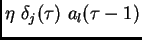 , where
  is the
learning rate, and
is the
learning rate, and  stands for an arbitrary unit
connected to unit .
stands for an arbitrary unit
connected to unit .
Next: Error path integral
Up: Exponential error decay
Previous: Exponential error decay
Juergen Schmidhuber
2003-02-19