Outline.
We are interested in weights representing nets
with tolerable error but flat outputs (see section 2 and appendix A.1).
To find nets with flat outputs,
two conditions will be defined
to specify ![]() for
for ![]() and, as a consequence,
and, as a consequence, ![]() (see section 3).
The first condition ensures flatness.
The second condition enforces ``equal flatness'' in all
weight space directions, to obtain low variance of the net
functions induced by weights within a box. The second
condition will be
justified using an MDL-based argument.
In both cases, linear approximations will be made
(to be justified in A.2).
(see section 3).
The first condition ensures flatness.
The second condition enforces ``equal flatness'' in all
weight space directions, to obtain low variance of the net
functions induced by weights within a box. The second
condition will be
justified using an MDL-based argument.
In both cases, linear approximations will be made
(to be justified in A.2).
Formal details. We are interested in weights causing tolerable error (see ``acceptable minima'' in section 2) that can be perturbed without causing significant output changes, thus indicating the presence of many neighboring weights leading to the same net function. By searching for the boxes from section 2, we are actually searching for low-error weights whose perturbation does not significantly change the net function.
In what follows we treat the input ![]() as fixed: for
convenience, we suppress
as fixed: for
convenience, we suppress ![]() , i.e. we abbreviate
, i.e. we abbreviate
![]() by
by ![]() .
Perturbing the weights
.
Perturbing the weights ![]() by
by
![]() (with components
(with components ![]() ),
we obtain
),
we obtain
![]() ,
where
,
where ![]() expresses
expresses ![]() 's
dependence on
's
dependence on ![]() (in what follows,
however,
(in what follows,
however, ![]() often will be suppressed for
convenience, i.e. we abbreviate
often will be suppressed for
convenience, i.e. we abbreviate ![]() by
by ![]() ).
Linear approximation (justified in A.2)
gives us ``Flatness Condition 1'':
).
Linear approximation (justified in A.2)
gives us ``Flatness Condition 1'':
Many boxes ![]() satisfy flatness condition 1.
To select a particular, very flat
satisfy flatness condition 1.
To select a particular, very flat ![]() ,
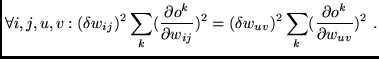
the following
``Flatness Condition 2''
uses up degrees of freedom
left by inequality (3):
,
the following
``Flatness Condition 2''
uses up degrees of freedom
left by inequality (3):
How to derive the algorithm from flatness conditions 1 and 2.
We first solve equation (4) for
 (fixing
 ![]() for all
for all ![]() ).
Then we insert the
).
Then we insert the
![]() (with fixed
(with fixed ![]() ) into inequality
(3)
(replacing the second ``
) into inequality
(3)
(replacing the second ``![]() '' in (3) by ``
'' in (3) by ``![]() '', since
we search for the box with maximal volume).
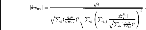
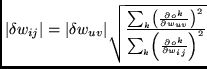
This gives us an equation for the
'', since
we search for the box with maximal volume).
This gives us an equation for the
![]() (which depend on
(which depend on
![]() , but this is notationally suppressed):
, but this is notationally suppressed):
The
![]() (
(![]() is replaced by
is replaced by ![]() ) approximate
the
) approximate
the ![]() from section 2. The box
from section 2. The box ![]() is approximated
by
is approximated
by ![]() , the box with center
, the box with center ![]() and edge lengths
and edge lengths
![]() .
.
![]() 's volume
's volume ![]() is approximated by
is approximated by ![]() 's box volume
's box volume
![]() .
Thus,
.
Thus,
![]() (see section 3) can be
approximated by
(see section 3) can be
approximated by
![]() .
This immediately leads to the algorithm given by
equation (1).
.
This immediately leads to the algorithm given by
equation (1).
How can the above approximations be justified? The learning process itself enforces their validity (see A.2). Initially, the conditions above are valid only in a very small environment of an ``initial'' acceptable minimum. But during search for new acceptable minima with more associated box volume, the corresponding environments are enlarged. Appendix A.2 will prove this for feedforward nets (experiments indicate that this appears to be true for recurrent nets as well).
Comments.
Flatness condition 2 influences
the algorithm as follows: (1) The algorithm prefers to
increase the ![]() 's of weights whose current
contributions are
not important to compute the target output.
(2) The algorithm enforces equal sensitivity of all
output units with respect to weights of connections to
hidden units. Hence, output units tend to share hidden
units, i.e., different hidden units tend to
contribute equally to the computation of the target. The
contributions of a particular hidden unit
to different output unit activations tend to be equal, too.
's of weights whose current
contributions are
not important to compute the target output.
(2) The algorithm enforces equal sensitivity of all
output units with respect to weights of connections to
hidden units. Hence, output units tend to share hidden
units, i.e., different hidden units tend to
contribute equally to the computation of the target. The
contributions of a particular hidden unit
to different output unit activations tend to be equal, too.
Flatness condition 2 is essential: flatness condition 1 by itself corresponds to nothing more but first order derivative reduction (ordinary sensitivity reduction). However, as mentioned above, what we really want is to minimize the variance of the net functions induced by weights near the actual weight vector.
Automatically, the algorithm treats units and weights in different layers differently, and takes the nature of the activation functions into account.