In a realistic application, of course, it is implausible to
assume that the errors of all ![]() are minimal at all times.
After having modified the functions computing the internal
representations, the
are minimal at all times.
After having modified the functions computing the internal
representations, the ![]() must be trained for some
time to assure that they can adapt to the new situation.
must be trained for some
time to assure that they can adapt to the new situation.
Each of the ![]() predictors, the
predictors, the ![]() representational
modules, and the potentially
available auto-associator can be
implemented as a feed-forward back-propagation
network (e.g. Werbos, 1974).
There are two alternating passes - one for minimizing
prediction errors, the other one for maximizing
representational
modules, and the potentially
available auto-associator can be
implemented as a feed-forward back-propagation
network (e.g. Werbos, 1974).
There are two alternating passes - one for minimizing
prediction errors, the other one for maximizing ![]() . Here
is an off-line version based on successive
`epochs' (presentations of the whole ensemble of training patterns):
. Here
is an off-line version based on successive
`epochs' (presentations of the whole ensemble of training patterns):
PASS 1 (minimizing prediction errors):
Repeat for a `sufficient' number of training epochs:
1. For all ![]() :
:
1.1. For all ![]() : Compute
: Compute ![]() .
.
1.2. For all ![]() : Compute
: Compute ![]() .
.
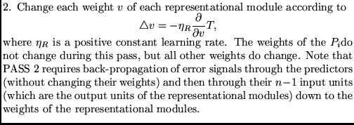
2. Change each weight ![]() of each
of each ![]() according to
according to
where ![]() is a positive constant learning rate.
is a positive constant learning rate.
PASS 2 (minimizing predictability):
2. For all ![]() :
:
2.1. For all ![]() : Compute
: Compute ![]() .
.
2.2. For all ![]() : Compute
: Compute ![]() .
.
2.3. If an auto-associator is involved, compute ![]() .
.
The off-line version above is perhaps not as appealing as a more local procedure where computing time is distributed evenly between PASS 2 and PASS 1:
An on-line version.
An extreme on-line version does not sweep
through the whole training ensemble before changing
weights. Instead it processes the same
single input pattern ![]() (randomly chosen according to
the input distribution) in both PASS 1 and PASS 2 and
immediately changes
the weights of all involved networks simultaneously, according to
the contribution of
(randomly chosen according to
the input distribution) in both PASS 1 and PASS 2 and
immediately changes
the weights of all involved networks simultaneously, according to
the contribution of ![]() to the respective objective functions.
to the respective objective functions.
Simultaneous updating of the representations and the predictors, however, introduces a potential for instabilities. Both the predictors and the representational modules perform gradient descent (or gradient ascent) in changing functions. Given a particular implementation of the basic principle, experiments are needed to find out how much on-line interaction is permittable. With the toy-experiments reported below, on-line learning did not cause major problems.
It should be noted that if
![]() (section 5), then
with a given input pattern
we may compute the gradient of
(section 5), then
with a given input pattern
we may compute the gradient of ![]() with respect to
both the predictor weights and the weights of the representation
modules in a single pass. After this we may simply perform
gradient descent in the predictor weights and gradient
ascent in the remaining weights (it is just a matter of
flipping signs). This was actually done in the
experiments.
with respect to
both the predictor weights and the weights of the representation
modules in a single pass. After this we may simply perform
gradient descent in the predictor weights and gradient
ascent in the remaining weights (it is just a matter of
flipping signs). This was actually done in the
experiments.
Local maxima.
Like all gradient ascent procedures, the method is subject
to the problem of local maxima.
A standard method for dealing with local maxima is to repeat
the above algorithm with different weight initializations
(using a fixed number ![]() of training epochs for each repetition)
until a (near-) factorial
code is found. Each repetition corresponds to a local search around
the point in weight space defined by the current weight
initialization.
of training epochs for each repetition)
until a (near-) factorial
code is found. Each repetition corresponds to a local search around
the point in weight space defined by the current weight
initialization.
Shared hidden units. It should be mentioned that some or all of the representational modules may share hidden units. The same holds for the predictors. Predictors sharing hidden units, however, will have to be updated sequentially: No representational unit may be used to predict its own activity.