PREDICTABILITY MINIMIZATION: DETAILS

In its most simple form, PM is based on a feedforward network with $n$ sigmoid output units (or code units). See Figure 1.

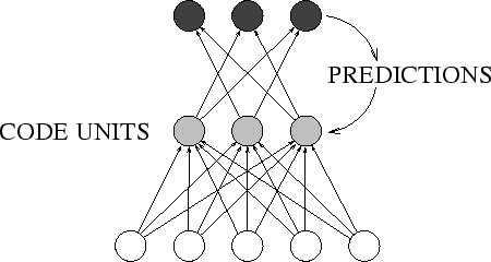
Figure 1: Predictability minimization (PM): input patterns with redundant components are coded across $n$ code units (grey). Code units are also input units of $n$ predictor networks. Each predictor (output units black) attempts to predict its code unit (which it cannot see). But each code unit tries to escape the predictions, by representing environmental properties that are independent from those represented by other code units. This encourages high information throughput and redundancy reduction. Predictors and code generating net may have hidden units. In this paper, however, they don't. See text for details.

The $i$-th code unit produces a real-valued output value $y^p_i \in [0, 1]$ (the unit interval) in response to the $p$-th external input vector $x^p$ (later we will see that training tends to make the ouput values near-binary). There are $n$ additional feedforward nets called predictors, each having one output unit and $n-1$ input units. The predictor for code unit $i$ is called $P_i$. Its real-valued output in response to the $\{ y_k^p :~~ k \neq i \}$ is called $P^p_i$. $P_i$ is trained (in our experiments by conventional online backprop) to minimize

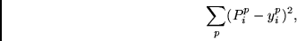$$\sum_p (P_i^p - y_i^p)^2,$$ (1)

thus learning to approximate the conditional expectation 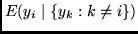$E(y_i \mid \{y_k: k \neq i \})$ of $y_i$, given the activations of the remaining code units. Of course, this conditional expectation typically will be very different from the actual activations of the code unit. For instance, assume that a certain code unit will be switched on in one third of all cases within a given context (defined by the activations of the remaining code units), while it will be switched off in two thirds of all such cases. Then, given this context, the predictor will predict a value of 0.3333.

The clue is: the code units are trained (in our experiments by online backprop) to maximize essentially the same objective function [Schmidhuber, 1992] the predictors try to minimize:

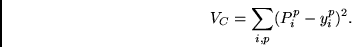$$V_C = \sum_{i,p}(P_i^p - y_i^p)^2.$$ (2)

Predictors and code units co-evolve by fighting each other.

Justification. Let us assume that the $P_i$ never get trapped in local minima and always perfectly learn the conditional expectations. It then turns out that the objective function $V_C$ is essentially equivalent to the following one (also given in Schmidhuber, 1992):

$$\sum_i VAR(y_i) -\sum_{i,p} (P^p_i - \bar{y_i})^2,$$ (3)

where $\bar{y_i}$ denotes the mean activation of unit $i$, and VAR denotes the variance operator. The equivalence of (2) and (3) was observed by Peter Dayan, Richard Zemel and Alex Pouget (personal communication, SALK Institute, 1992 -- see [Schmidhuber, 1993] for details). (3) gives some intuition about what is going on while (2) is maximized. Mazimizing the first term of (3) tends to enforce binary units, and also local maximization of information throughput (given the binary constraint). Maximizing the second (negative) term (or minimizing the corresponding unsigned term) tends to make the conditional expectations equal to the unconditional expectations, thus encouraging mutual statistical independence (zero mutual information) and global maximization of information throughput.

Back to Independent Component Analysis page.