Table 1 gives an overview of various time-dependent activation vectors
relevant for the description of the algorithm. Additional notation:
`![]() ' is the concatenation operator;
' is the concatenation operator;
![]() if the teacher provides a target vector
if the teacher provides a target vector
![]() at time
at time ![]() and
and
![]() otherwise.
If
otherwise.
If
![]() then
then ![]() takes on some default value,
e.g. the zero vector.
takes on some default value,
e.g. the zero vector.
------------INSERT TABLE 1 HERE--------------
|
A has ![]() input units,
input units,
![]() hidden units, and
hidden units, and
![]() output units (see table 1).
With pure prediction tasks
output units (see table 1).
With pure prediction tasks
![]() .
C has
.
C has
![]() hidden units, and
hidden units, and
![]() output units.
All of A's input and hidden units
have directed connections to
all of A's hidden and output units.
All input units
of A have directed connections to
all hidden and output units of C. This is because A's
input units
serve as input units for C
at certain time steps. There are additional
output units.
All of A's input and hidden units
have directed connections to
all of A's hidden and output units.
All input units
of A have directed connections to
all hidden and output units of C. This is because A's
input units
serve as input units for C
at certain time steps. There are additional
![]() input units for C for providing unique representations
of the current time step.
These additional input units also have directed connections to
all hidden and output units of C.
All hidden units
of C have directed connections to
all hidden and output units of C.
input units for C for providing unique representations
of the current time step.
These additional input units also have directed connections to
all hidden and output units of C.
All hidden units
of C have directed connections to
all hidden and output units of C.
A will try to make
![]() equal to
equal to ![]() if
if ![]() , and
it will try to make
, and
it will try to make
![]() equal to
equal to ![]() , thus trying to predict
, thus trying to predict ![]() .
Here again the target prediction problem is defined as a special case
of an input prediction problem.
C will try to make
.
Here again the target prediction problem is defined as a special case
of an input prediction problem.
C will try to make
![]() equal to the externally provided teaching vector
equal to the externally provided teaching vector ![]() if
if ![]() and if A failed to emit
and if A failed to emit ![]() .
Furthermore, it will always try to make
.
Furthermore, it will always try to make
![]() equal to
the next non-teaching input to be processed
by C. This input may be many time steps ahead.
Finally, and most importantly, A will try to make
equal to
the next non-teaching input to be processed
by C. This input may be many time steps ahead.
Finally, and most importantly, A will try to make
![]() equal to
equal to
![]() , thus trying to predict the
state of C. The activations of C's
output units are considered
as part of its state.
, thus trying to predict the
state of C. The activations of C's
output units are considered
as part of its state.
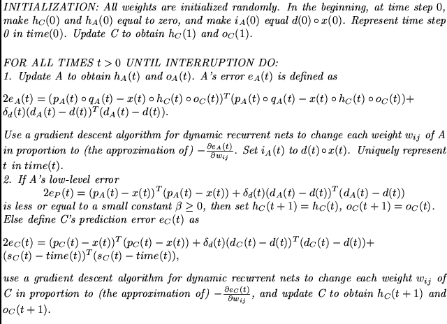
Both C and A simultaneously are trained by a conventional algorithm for recurrent networks in an on-line fashion. Both the IID-Algorithm and BPTT are appropriate. In particular, computationally inexpensive variants of BPTT [Williams and Peng, 1990] are interesting: There are tasks with hierarchical temporal structure where only a few iterations of `back-propagation back into time' per time step are in principle sufficient to bridge arbitrary time lags (see section 5).
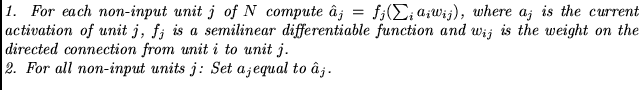
I now describe the (quite familiar) procedure for updating activations in a net.
Repeat for a constant number of iterations (typically one or two):
I now specify the input-output behavior of the chunker and the automatizer as well as the details of error injection: