26 March 1991: Neural nets learn to program neural nets with fast weights—like today's Transformer variants. 2021: New stuff!
Abstract.
How can artificial neural networks (NNs) process sequential data such as videos, speech, and text?
Traditionally this is done with recurrent NNs (RNNs)
that learn to remember past observations.
Exactly 3 decades ago, however,
a now very popular
alternative to RNNs was
published.[FWP0-1]
A feedforward NN slowly learns by gradient descent to program the changes of
the fast weights of
another NN (see Sec. 1).
Such Fast Weight Programmers (FWPs) can learn to memorize past data, too.
In 1991, one of them[FWP0-1]
computed its fast weight changes through
additive outer products of self-invented activation patterns
(now often called keys and values for self-attention; Sec. 2).
The very similar Transformers[TR1-2] combine this with projections
and softmax and
are now widely used in natural language processing.
For long input sequences, their efficiency was improved through
linear Transformers or Performers[TR5-6]
whose core is formally equivalent to the 1991 Fast Weight Programmers.
In 1993, I introduced
the attention terminology[FWP2] now used
in this context[ATT] (Sec. 4), and
extended the approach to
RNNs that program themselves
(Sec. 3).
FWPs can solve the
famous vanishing gradient
problem aka deep learning problem (analyzed a few months later in 1991[VAN1])
through additive fast weight changes (Sec. 5).
This is symmetric to the
additive neural activations of LSTMs / Highway Nets / ResNets[HW1-3] (Sec. 5)
which also have roots in 1991—the
Annus Mirabilis of deep learning.[MIR]
In 2021, we introduced a
brand new, improved version[FWP6] of
the 1991 fast weight update rule (Sec. 6).
As an addendum,
I also review our
FWPs for
reinforcement learning through neuroevolution[FWP5] (2005-, Sec. 7)
and for
metalearning machines that learn to learn[FWPMETA1-7]
(1992-, Sec. 8).
 As I have frequently emphasized since 1990,[AC90][PLAN][META]
the connection strengths or weights of
an
artificial neural network (NN)
should be viewed as its program.
Inspired by
Gödel's
universal self-referential formal systems,[GOD][GOD34]
I built NNs whose outputs are changes of programs or weight matrices of other NNs[FWP0-2]
(Sec. 1, 2, 3),
and even self-referential recurrent NNs (RNNs)
that can run and inspect and modify
their own weight change algorithms or learning algorithms[FWPMETA1-5] (Sec. 8).
A difference to Gödel's work was that my universal programming language was not based on the integers,
but on real-valued weights:
each NN's output is differentiable with respect to its program.
That is, a simple program generator (the efficient
gradient descent procedure[BP1-4][BPA][R7])
can compute a direction in program space where one may find a better program,[AC90]
in particular, a
better program-modifying program.[FWP0-2][FWPMETA1-5]
Much of my work since 1989 has exploited this fact.
As I have frequently emphasized since 1990,[AC90][PLAN][META]
the connection strengths or weights of
an
artificial neural network (NN)
should be viewed as its program.
Inspired by
Gödel's
universal self-referential formal systems,[GOD][GOD34]
I built NNs whose outputs are changes of programs or weight matrices of other NNs[FWP0-2]
(Sec. 1, 2, 3),
and even self-referential recurrent NNs (RNNs)
that can run and inspect and modify
their own weight change algorithms or learning algorithms[FWPMETA1-5] (Sec. 8).
A difference to Gödel's work was that my universal programming language was not based on the integers,
but on real-valued weights:
each NN's output is differentiable with respect to its program.
That is, a simple program generator (the efficient
gradient descent procedure[BP1-4][BPA][R7])
can compute a direction in program space where one may find a better program,[AC90]
in particular, a
better program-modifying program.[FWP0-2][FWPMETA1-5]
Much of my work since 1989 has exploited this fact.
Successful learning in deep architectures
started in 1965
when
Ivakhnenko & Lapa published the first general, working learning algorithms for deep multilayer perceptrons with arbitrarily many hidden layers.[DEEP1-2] Their activation functions were Kolmogorov-Gabor polynomials which include the now popular multiplicative gates,[DL1][DL2]
an important ingredient of later NNs with
dynamic links or
fast weights.
In 1981,
von der Malsburg was the first to explicitly emphasize the importance of NNs with rapidly changing weights.[FAST] The second paper on this was published by Feldman in 1982.[FASTa]
The weights of a 1987 NN were sums of weights with a large learning rate and weights with a small rate[FASTb][T20] (but have nothing to do with the NN-programming NNs discussed below).
Before 1991, no network learned by gradient descent to quickly compute the changes of the fast weight storage of another network or of itself. Such
Fast Weight Programmers (FWPs) were published in 1991-93[FWP0-2]
(Sec. 1, 2, 3, 4).
They embody the principles found in certain types of what is now called
attention[ATT] (Sec. 4)
and Transformers[TR1-6]
(Sec. 2, 3, 4, 5).
1. 1991: NNs learn to program other NNs, separating storage and control
 Three decades ago,
on 26 March 1991,
I described a sequence-processing
slow NN that learns by backpropagation[BP1-4] to rapidly modify
the fast weights of another NN,[FWP0] essentially
by adding or subtracting (possibly large) values to the fast weights at each time step of the sequence.
This was later also
published
in Neural Computation.[FWP1]
The slow NN learns to control or program the weights of the fast NN,
such that the fast NN can quickly refocus its
attention[ATT]
(Sec. 4)
on particular aspects of the
incoming stream of input observations.
Three decades ago,
on 26 March 1991,
I described a sequence-processing
slow NN that learns by backpropagation[BP1-4] to rapidly modify
the fast weights of another NN,[FWP0] essentially
by adding or subtracting (possibly large) values to the fast weights at each time step of the sequence.
This was later also
published
in Neural Computation.[FWP1]
The slow NN learns to control or program the weights of the fast NN,
such that the fast NN can quickly refocus its
attention[ATT]
(Sec. 4)
on particular aspects of the
incoming stream of input observations.
That is, I separated storage and control like in traditional computers,
but in a fully neural way (rather than in a hybrid fashion[PDA1][PDA2][DNC]).
Compare my related work of 1990 on
what's now sometimes called
Synthetic Gradients.[NAN1-5]
The slow NN does not simply overwrite the current fast weights,
but changes them in a way that takes their past values into account.
That is, although both NNs are of the feedforward type,
they can solve tasks that normally only
recurrent NNs (RNNs)
can solve,
since the slow NN can program the fast weights to implement a short-term memory of certain previous events.
This so-called short-term memory may actually last for a long time—see Sec. 5.
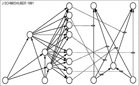
One of the FWPs of 1991[FWP0-1] is illustrated in the figure. There is
a separate output unit of the slow net for each connection of the fast net.
While processing a data sequence,
the slow net can quickly reprogram the mapping from inputs to outputs implemented by the fast net.
A disadvantage addressed in Sec. 2 is that the slow net needs many output units if the fast net is large.
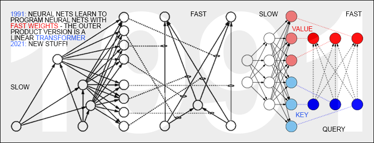
2. NNs program NNs through outer products: core of linear Transformers
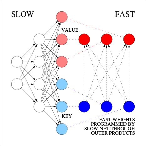
The Fast Weight Programmer[FWP0-1] depicted in Sec. 1 has a slow net unit for each fast weight.
However, Section 2 of the same 1991 paper[FWP0]
also describes a more efficient approach which has become the core principle of
linear[TR5-6] Transformers[TR1-2] or
attention[ATT] (compare Sec. 4).
Here the slow net has a special unit for each fast net
unit from which at least one fast connection is originating. The set of these units is called
FROM (blue in the image).
The slow net also has a special unit for each fast net unit to which at least one fast connection is leading. The set of these units is called TO (red in the image). At every time step of sequence processing, each fast weight may rapidly change in proportion to the product of the current activations of the corresponding units in FROM and TO. This product is simply added
to the fast weight (which then may be normalized by a squashing function[FWP0]). The
additive part by itself essentially
overcomes the vanishing gradient problem—see Sec. 5.
In today's Transformer terminology,
FROM and TO are called
key and value, respectively.
The INPUT to which the fast net is applied is called the query.
Essentially, the query is processed by the fast weight matrix, which is
a sum of outer products of keys
and values (ignoring normalizations and projections).
Since all operations of both networks are differentiable, we obtain end-to-end differentiable
active control of fast weight changes through additive outer products or
second order tensor products.[FWP0-3a]
Hence the slow net can learn by gradient descent to rapidly modify the fast net during sequence processing.
This is mathematically equivalent (apart from normalization) to what was later called
linear Transformers.[FWP6][TR5-6]
The highly successful Transformers of 2017[TR1-2] can be viewed as a combination of my
additive outer product fast weight principle[FWP0-2]
and softmax:
attention (query, key, value) ~ softmax (query key) value.
The attention weights in Transformers
can be viewed as context-dependent weight vectors or
NN-programmed fast weights (Sec. 5 & 1).
In the interest of efficiency,
linear Transformers (2020-21)[TR5-6]
abandoned the softmax, essentially resurrecting the original 1991 system.[FWP0-1] Compare Sec. 6.
Of course, plain outer products in NNs
go back at least to Hebb's informal rule (1949)[HE49] and
concrete formal implementations through
Steinbuch's Learning Matrix around 1960.[ST61-63][KOH72][LIT74][PAL80][HO82][KOS88]
However, these authors described pre-wired rules to
associate given patterns with each other. Their
systems did not learn to use such rules for
associating self-invented patterns like the FWPs
since 1991.[FWP0-3a][TR5-6]
The latter are essentially NN-programming NNs
whose elementary programming instructions
are additive outer product rules.
The NNs must learn to use the rules wisely to achieve their goals.
I offered the FWPs of 1991[FWP0-1] as an
alternative to
sequence-processing recurrent NNs (RNNs)
(Sec. 1),
the computationally most powerful NNs of them all.[UN][MIR](Sec. 0)
Modern Transformers are also viewed as RNN alternatives, despite their limitations.[TR3-4]
3. Core principles of recurrent linearized Transformers in 1993
The slow net and the fast net of the 1991 system[FWP0-1] in Sec. 2 were feedforward NNs (FNNs),
like most current Transformers.[TR1-6]
In 1993, however, to combine the best of both recurrent NNs (RNNs) and fast weights,
I collapsed all of this into a single RNN that could rapidly
reprogram all of its own fast weights through additive outer product-based weight changes.[FWP2]
One motivation reflected by the title of the paper[FWP2]
was to get many more temporal variables under massively parallel end-to-end differentiable control than what's possible in standard RNNs of the same size: O(H2) instead of O(H), where H is the number of hidden units. This motivation and a variant of the method was republished over two decades later.[FWP4a][R4][MIR](Sec. 8)[T20](Sec. XVII; item 7)
See also our more recent work on FWPs since 2017,[FWP3-3a][FWPMETA7][FWP6] and compare a recent study.[RA21]
 Today, everybody is talking about attention when it comes to describing the principles of Transformers.[TR1-2]
The additive outer products[FWP0-1] of the Fast Weight Programmers described
in Sec. 2 and Sec. 3
are often viewed as attention layers.
Similarly, the attention weights or self-attention weights (see also[FWP4b-d])
in Transformers
can be viewed as context-dependent weight vectors or
NN-programmed fast weights (Sec. 5).[FWP0-1], Sec. 9 & Sec. 8 of [MIR], Sec. XVII of [T20]
Today, everybody is talking about attention when it comes to describing the principles of Transformers.[TR1-2]
The additive outer products[FWP0-1] of the Fast Weight Programmers described
in Sec. 2 and Sec. 3
are often viewed as attention layers.
Similarly, the attention weights or self-attention weights (see also[FWP4b-d])
in Transformers
can be viewed as context-dependent weight vectors or
NN-programmed fast weights (Sec. 5).[FWP0-1], Sec. 9 & Sec. 8 of [MIR], Sec. XVII of [T20]
This kind of attention-oriented terminology was introduced in my
1993 paper[FWP2] which
explicitly mentioned the learning of
internal spotlights of attention
in its additive outer product-based (or second order tensor product-based)
Fast Weight Programmers.[FWP2][ATT]
5. Dual additive paths towards deep learning: LSTM v fast weight programs
Apart from possible normalization/squashing,[FWP0]
the 1991 Fast Weight Programmer's weight changes
are additive (Sec. 1 & 2).
Additive FWPs
do not suffer during sequence learning from the famous vanishing gradient
problem aka deep learning problem.
In fact, they embody a solution to this problem which was first analyzed
by my brilliant student Sepp Hochreiter a few months later in his 1991 diploma thesis.[VAN1]
 It turns out that the problem
can be solved in two closely related ways, both of them based on additive control of temporal storage,
and both of them dating back to 1991, our miraculous year of deep learning.[MIR]
It turns out that the problem
can be solved in two closely related ways, both of them based on additive control of temporal storage,
and both of them dating back to 1991, our miraculous year of deep learning.[MIR]
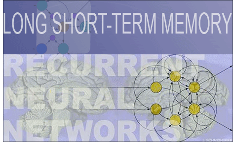
Basic Long Short-Term Memory[LSTM1] solves the problem by adding at every time step
new real values to old internal neural activations
through recurrent connections whose weights are always 1.0.
That is, the core of LSTM is operating in a linear additive activation space (ignoring LSTM's multiplicative gates).[LSTM1][VAN1][MIR](Sec. 4 & Sec. 8)
Additive FWPs[FWP0-2] (Sec. 1 & 2), however, solve the problem through a dual approach,
namely, by adding real values to fast weights (rather than neuron activations).
That is, they are operating in an additive fast weight space.
Since the fundamental operation of NNs is to multiply weights by activations, both approaches are symmetric.
By favoring additive operations yielding non-vanishing first derivatives and error flow,[VAN1]
both are in principle immune to the vanishing gradient problem, for the same reason.
Since 2017,
Transformers[TR1-6]
also follow the additive approach.[FWP0-2]
Their context-dependent attention weights
used for weighted averages of value vectors
are like NN-programmed fast weights that change for each new input
(compare Sec. 2 and Sec. 4 on attention terminology since 1993).
 LSTM's traditional additive activation-based approach[LSTM1-13]
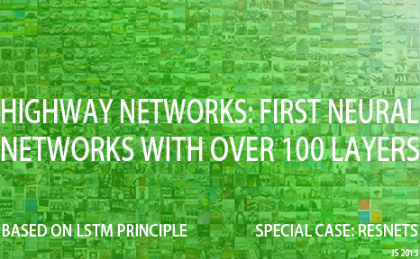
is mirrored in the LSTM-inspired Highway Network (May 2015),[HW1][HW1a][HW3] the first working really deep
feedforward neural network with hundreds of layers.
It is essentially a feedforward version of LSTM[LSTM1] with forget gates.[LSTM2]
If we open its gates (and keep them open),
we obtain a special case called
Residual Net or ResNet[HW2] (Dec 2015).
LSTM's traditional additive activation-based approach[LSTM1-13]
is mirrored in the LSTM-inspired Highway Network (May 2015),[HW1][HW1a][HW3] the first working really deep
feedforward neural network with hundreds of layers.
It is essentially a feedforward version of LSTM[LSTM1] with forget gates.[LSTM2]
If we open its gates (and keep them open),
we obtain a special case called
Residual Net or ResNet[HW2] (Dec 2015).
In sum, to solve the deep learning problem through additive control of some NN's internal storage,
we may use either the family of additive Fast Weight Programmers / (linear) Transformers,
or the dual family of LSTM / Highway Nets / ResNets.
The former are easily parallelizable.
Remarkably, both of these dual approaches of 1991 have become successful.
By
the mid 2010s,[DEC]
all the
major IT companies overwhelmingly used
LSTMs for speech recognition, natural language processing (NLP), machine translation,
and many other AI applications. For example, LSTMs were used for translating texts many billions of times per day on billions of smartphones.[DL4]
In recent years, however,
Transformers have
excelled at the traditional LSTM domain of
NLP[TR1-2]—although there are still many language tasks that LSTM can
rapidly learn to solve quickly[LSTM13]
while plain Transformers can't yet.[TR4]
An orthogonal approach to solving the deep learning problem is based on
unsupervised pre-training of deep NNs.[UN0-UN2][MIR](Sec. 1)
Remarkably, this approach
also
dates back to 1991[UN]
(which happens to be the only palindromic year of the 20th century).
6. Most recent work on fast weight-based Transformers (2021)
Recent work of February 2021[FWP6]
with my PhD student Imanol Schlag and my postdoc Kazuki Irie not only
emphasizes the formal equivalence of linear Transformer-like self-attention
mechanisms[TR5-6] and Fast Weight Programmers[FWP0-2]
(Sec. 2).[FWP4a][R4][MIR](Sec. 8)[T20](Sec. XVII; item 7)
We also infer a memory capacity
limitation of recent linearized softmax attention
variants.[TR5-6] With finite memory, a desirable behavior
of FWPs is to manipulate
the contents of memory and dynamically interact
with it. Building on previous work[FWPMETA7] on FWPs
(Sec. 1, 2, 3, 8),
we replace the 1991 update rule[FWP0-2] by an alternative
rule yielding such behavior. We also
introduce a new kernel function to linearize attention,
balancing simplicity and effectiveness. To demonstrate the
benefits of our methods, we
conduct experiments on synthetic retrieval problems
as well as standard machine translation and
language modeling tasks.[FWP6]
7. Fast weights for reinforcement learning / neuroevolution (2005)
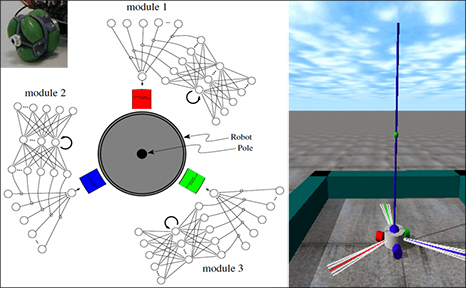
Deep reinforcement learning (RL) without a teacher can
profit from fast weights even when the environment's dynamics are not differentiable,
as shown in 2005
with my former postdoc Faustino Gomez[FWP5]
(now CEO of NNAISENSE)
when affordable computers were about 1000 times faster than in the early 1990s.
For example, a robot with three wheels controlled by a Fast Weight Programmer
learned to balance a pole topped by another pole.
In the past 3 decades we have published quite a few additional ways of learning to quickly generate
numerous weights of large NNs through very compact codes.[KO0-2][CO1-4] Here we exploited that the
Kolmogorov complexity or algorithmic information content of successful huge NNs may actually be rather small.
For example, in July 2013, the compact codes of
Compressed Network Search[CO2]
yielded the
first deep learning model to successfully learn control policies directly from high-dimensional
sensory input (video) using RL (in this case RL through neuroevolution),
without any
unsupervised pre-training.
8. Metalearning with Fast Weight Programmers
 My first work on metalearning machines that
learn to learn was published in 1987.[META][R3]
Five years later, I showed how Fast Weight Programmers can also be used for
metalearning in a very general way.
In references[FWPMETA1-5] since 1992, the slow NN and the fast NN
(Sec. 1) are recurrent and identical.
The RNN can see its own errors or reward signals called eval(t+1) in the image.[FWPMETA5]
The initial weight of each connection is trained by gradient descent, but during a training episode, each connection can be addressed
and read and modified by the RNN itself through O(log n) special output units, where n is the number of connections—see time-dependent vectors mod(t), anal(t), Δ(t), val(t+1) in the image. That is, each connection's weight may rapidly change, and the network becomes self-referential in the sense that it can in principle run arbitrary computable weight change algorithms or learning algorithms (for all of its weights) on itself.
My first work on metalearning machines that
learn to learn was published in 1987.[META][R3]
Five years later, I showed how Fast Weight Programmers can also be used for
metalearning in a very general way.
In references[FWPMETA1-5] since 1992, the slow NN and the fast NN
(Sec. 1) are recurrent and identical.
The RNN can see its own errors or reward signals called eval(t+1) in the image.[FWPMETA5]
The initial weight of each connection is trained by gradient descent, but during a training episode, each connection can be addressed
and read and modified by the RNN itself through O(log n) special output units, where n is the number of connections—see time-dependent vectors mod(t), anal(t), Δ(t), val(t+1) in the image. That is, each connection's weight may rapidly change, and the network becomes self-referential in the sense that it can in principle run arbitrary computable weight change algorithms or learning algorithms (for all of its weights) on itself.
The 1993 FWP of Sec. 3[FWP2] also was an RNN
that could quickly manipulate all of its own weights. However, unlike the self-referential
RNN above,[FWPMETA1-5]
it used outer products between key patterns and value patterns (Sec. 2) to manipulate
many fast weights in parallel.
In 2001,
Sepp et al.
used gradient descent in LSTM networks[LSTM1] instead of traditional
RNNs to metalearn
fast online learning
algorithms for nontrivial classes of functions, such as all quadratic
functions of two variables[HO1] (more on LSTM and fast weights in Sec. 5).
In 2020, Imanol et al. augmented an LSTM with an associative fast weight memory.[FWPMETA7] Through differentiable operations at every step of a given input sequence, the LSTM updates and maintains compositional associations of former observations stored in the rapidly changing fast weights. The model is trained end-to-end by gradient descent and yields excellent performance on compositional language reasoning problems, small-scale word-level language modelling, and meta-RL for
partially observable environments.[FWPMETA7]
Our recent MetaGenRL (2020)[METARL10] meta-learns
novel RL algorithms applicable to environments that significantly differ from those used for training.
MetaGenRL searches the space of low-complexity loss functions that describe such learning algorithms.
See the blog post of my PhD student Louis Kirsch.
This principle of searching for simple learning algorithms is also applicable to fast weight architectures.
Using weight sharing and sparsity, our recent Variable Shared Meta Learning (VS-ML) implicitly creates
outer-product-like fast weights encoded in the activations of LSTMs.[FWPMETA6]
This allows for encoding the learning algorithm by few parameters although it has many time-varying
variables[FWP2] (Sec. 3).
Some of these activations can be interpreted as NN weights updated by the LSTM dynamics.
LSTMs with shared sparse entries in their weight matrix discover learning algorithms that generalize to new datasets.
The meta-learned learning algorithms do not require explicit gradient calculation.
VS-ML can also learn to implement the backpropagation learning algorithm[BP1-4]
purely in the end-to-end differentiable forward dynamics of RNNs.[FWPMETA6]
Acknowledgments
Thanks to several expert reviewers for useful comments. Since science is about self-correction, let me know under juergen@idsia.ch if you can spot any remaining error.
There is another version of this article with references in plain text style.
The contents of this article may be used for educational and non-commercial purposes, including articles for Wikipedia and similar sites.
This work is licensed under a Creative Commons Attribution-NonCommercial-ShareAlike 4.0 International License.

References
[GOD]
K. Gödel. Über formal unentscheidbare Sätze der Principia Mathematica und verwandter Systeme I. Monatshefte für Mathematik und Physik, 38:173-198, 1931.
[In the early 1930s, Gödel founded theoretical computer science. He identified fundamental limits of mathematics and theorem proving and computing and Artificial Intelligence.]
[GOD34]
K. Gödel (1934).
On undecidable propositions of formal mathematical
systems. Notes by S. C. Kleene and J. B. Rosser on lectures
at the Institute for Advanced Study, Princeton, New Jersey, 1934, 30
pp. (Reprinted in M. Davis, (ed.), The Undecidable. Basic Papers on Undecidable
Propositions, Unsolvable Problems, and Computable Functions,
Raven Press, Hewlett, New York, 1965.)
[Gödel introduced the first universal coding language.]
[AC90]
J. Schmidhuber.
Making the world differentiable: On using fully recurrent
self-supervised neural networks for dynamic reinforcement learning and
planning in non-stationary environments.
Technical Report FKI-126-90, TUM, Feb 1990, revised Nov 1990.
PDF
[FAST] C. v.d. Malsburg. Tech Report 81-2, Abteilung f. Neurobiologie,
Max-Planck Institut f. Biophysik und Chemie, Goettingen, 1981.
[First paper on fast weights or dynamic links.]
[FASTa]
J. A. Feldman. Dynamic connections in neural networks.
Biological Cybernetics, 46(1):27-39, 1982.
[2nd paper on fast weights.]
[FASTb]
G. E. Hinton, D. C. Plaut. Using fast weights to deblur old memories. Proc. 9th annual conference of the Cognitive Science Society (pp. 177-186), 1987.
[Two types of weights with different learning rates.]
[FWP0]
J. Schmidhuber.
Learning to control fast-weight memories: An alternative to recurrent nets.
Technical Report FKI-147-91, Institut für Informatik, Technische
Universität München, 26 March 1991.
PDF.
[First paper on fast weight programmers: a slow net learns by gradient descent to compute weight changes of a fast net.]
[FWP1] J. Schmidhuber. Learning to control fast-weight memories: An alternative to recurrent nets. Neural Computation, 4(1):131-139, 1992.
PDF.
HTML.
Pictures (German).
[FWP2] J. Schmidhuber. Reducing the ratio between learning complexity and number of time-varying variables in fully recurrent nets. In Proceedings of the International Conference on Artificial Neural Networks, Amsterdam, pages 460-463. Springer, 1993.
PDF.
[First recurrent fast weight programmer based on outer products.]
[FWP3] I. Schlag, J. Schmidhuber. Gated Fast Weights for On-The-Fly Neural Program Generation. Workshop on Meta-Learning, @N(eur)IPS 2017, Long Beach, CA, USA.
[FWP3a] I. Schlag, J. Schmidhuber. Learning to Reason with Third Order Tensor Products. Advances in Neural Information Processing Systems (N(eur)IPS), Montreal, 2018.
Preprint: arXiv:1811.12143. PDF.
[FWP4a] J. Ba, G. Hinton, V. Mnih, J. Z. Leibo, C. Ionescu. Using Fast Weights to Attend to the Recent Past. NIPS 2016.
PDF.
[FWP4b]
D. Bahdanau, K. Cho, Y. Bengio (2014).
Neural Machine Translation by Jointly Learning to Align and Translate. Preprint arXiv:1409.0473 [cs.CL].
[FWP4d]
Y. Tang, D. Nguyen, D. Ha (2020).
Neuroevolution of Self-Interpretable Agents.
Preprint: arXiv:2003.08165.
[FWP5]
F. J. Gomez and J. Schmidhuber.
Evolving modular fast-weight networks for control.
In W. Duch et al. (Eds.):
Proc. ICANN'05,
LNCS 3697, pp. 383-389, Springer-Verlag Berlin Heidelberg, 2005.
PDF.
HTML overview.
[Reinforcement-learning fast weight programmer.]
[FWP6] I. Schlag, K. Irie, J. Schmidhuber.
Linear Transformers Are Secretly Fast Weight Memory Systems. 2021. Preprint: arXiv:2102.11174.
[FWPMETA1] J. Schmidhuber. Steps towards `self-referential' learning. Technical Report CU-CS-627-92, Dept. of Comp. Sci., University of Colorado at Boulder, November 1992.
[First recurrent fast weight programmer that can learn
to run a learning algorithm or weight change algorithm on itself.]
[FWPMETA2] J. Schmidhuber. A self-referential weight matrix.
In Proceedings of the International Conference on Artificial
Neural Networks, Amsterdam, pages 446-451. Springer, 1993.
PDF.
[FWPMETA3] J. Schmidhuber.
An introspective network that can learn to run its own weight change algorithm. In Proc. of the Intl. Conf. on Artificial Neural Networks,
Brighton, pages 191-195. IEE, 1993.
[FWPMETA4]
J. Schmidhuber.
A neural network that embeds its own meta-levels.
In Proc. of the International Conference on Neural Networks '93,
San Francisco. IEEE, 1993.
[FWPMETA5]
J. Schmidhuber. Habilitation thesis, TUM, 1993. PDF.
[A recurrent neural net with a self-referential, self-reading, self-modifying weight matrix
can be found here.]
[FWPMETA6]
L. Kirsch and J. Schmidhuber. Meta Learning Backpropagation & Improving It. Metalearning Workshop at NeurIPS, 2020.
Preprint arXiv:2012.14905 [cs.LG], 2020.
[FWPMETA7]
I. Schlag, T. Munkhdalai, J. Schmidhuber.
Learning Associative Inference Using Fast Weight Memory.
To appear at ICLR 2021.
Report arXiv:2011.07831 [cs.AI], 2020.
[HO1]
S. Hochreiter, A. S. Younger, P. R. Conwell (2001). Learning to Learn Using Gradient Descent.
ICANN 2001. Lecture Notes in Computer Science, 2130, pp. 87-94.
[PDA1]
G.Z. Sun, H.H. Chen, C.L. Giles, Y.C. Lee, D. Chen. Neural Networks with External Memory Stack that Learn Context - Free Grammars from Examples. Proceedings of the 1990 Conference on Information Science and Systems, Vol.II, pp. 649-653, Princeton University, Princeton, NJ, 1990.
[PDA2]
M. Mozer, S. Das. A connectionist symbol manipulator that discovers the structure of context-free languages. Proc. N(eur)IPS 1993.
[DNC] Hybrid computing using a neural network with dynamic external memory.
A. Graves, G. Wayne, M. Reynolds, T. Harley, I. Danihelka, A. Grabska-Barwinska, S. G. Colmenarejo, E. Grefenstette, T. Ramalho, J. Agapiou, A. P. Badia, K. M. Hermann, Y. Zwols, G. Ostrovski, A. Cain, H. King, C. Summerfield, P. Blunsom, K. Kavukcuoglu, D. Hassabis.
Nature, 538:7626, p 471, 2016.
[NAN1]
J. Schmidhuber.
Networks adjusting networks.
In J. Kindermann and A. Linden, editors, Proceedings of
`Distributed Adaptive Neural Information Processing', St.Augustin, 24.-25.5.
1989, pages 197-208. Oldenbourg, 1990.
Extended version: TR FKI-125-90 (revised),
Institut für Informatik, TUM.
PDF.
[NAN2]
J. Schmidhuber.
Networks adjusting networks.
Technical Report FKI-125-90, Institut für Informatik,
Technische Universität München. Revised in November 1990.
PDF.
[NAN3]
J. Schmidhuber.
Recurrent networks adjusted by adaptive critics.
In Proc. IEEE/INNS International Joint Conference on Neural
Networks, Washington, D. C., volume 1, pages 719-722, 1990.
[NAN4]
J. Schmidhuber.
Additional remarks on G. Lukes' review of Schmidhuber's paper
`Recurrent networks adjusted by adaptive critics'.
Neural Network Reviews, 4(1):43, 1990.
[NAN5]
M. Jaderberg, W. M. Czarnecki, S. Osindero, O. Vinyals, A. Graves, D. Silver, K. Kavukcuoglu.
Decoupled Neural Interfaces using Synthetic Gradients.
Preprint arXiv:1608.05343, 2016.
[META1]
J. Schmidhuber.
Evolutionary principles in self-referential learning, or on learning
how to learn: The meta-meta-... hook. Diploma thesis,
Institut für Informatik, Technische Universität München, 1987.
Searchable PDF scan (created by OCRmypdf which uses
LSTM).
HTML.
[For example,
Genetic Programming
(GP) is applied to itself, to recursively evolve
better GP methods through Meta-Evolution. More.]
[METARL10]
L. Kirsch, S. van Steenkiste, J. Schmidhuber. Improving Generalization in Meta Reinforcement Learning using Neural Objectives. International Conference on Learning Representations, 2020.
[VAN1] S. Hochreiter. Untersuchungen zu dynamischen neuronalen Netzen. Diploma thesis, TUM, 15 June 1991 (advisor J. Schmidhuber). PDF.
[LSTM1] S. Hochreiter, J. Schmidhuber. Long Short-Term Memory. Neural Computation, 9(8):1735-1780, 1997. PDF.
More.
[LSTM2] F. A. Gers, J. Schmidhuber, F. Cummins. Learning to Forget: Continual Prediction with LSTM. Neural Computation, 12(10):2451-2471, 2000.
PDF.
[The "vanilla LSTM architecture" that everybody is using today, e.g., in Google's Tensorflow.]
[LSTM13]
F. A. Gers and J. Schmidhuber.
LSTM Recurrent Networks Learn Simple Context Free and
Context Sensitive Languages.
IEEE Transactions on Neural Networks 12(6):1333-1340, 2001.
PDF.
[HW1] R. K. Srivastava, K. Greff, J. Schmidhuber. Highway networks.
Preprints arXiv:1505.00387 (May 2015) and arXiv:1507.06228 (July 2015). Also at NIPS 2015. The first working very deep feedforward nets with over 100 layers. Let g, t, h, denote non-linear differentiable functions. Each non-input layer of a highway net computes g(x)x + t(x)h(x), where x is the data from the previous layer. (Like LSTM with forget gates[LSTM2] for RNNs.) Resnets[HW2] are a special case of this where the gates are always open: g(x)=t(x)=const=1.
Highway Nets perform roughly as well as ResNets[HW2] on ImageNet.[HW3] Highway layers are also often used for natural language processing, where the simpler residual layers do not work as well.[HW3]
More.
[HW1a]
R. K. Srivastava, K. Greff, J. Schmidhuber. Highway networks. Presentation at the Deep Learning Workshop, ICML'15, July 10-11, 2015.
Link.
[HW2] He, K., Zhang,
X., Ren, S., Sun, J. Deep residual learning for image recognition. Preprint
arXiv:1512.03385
(Dec 2015). Residual nets are a special case of Highway Nets[HW1]
where the gates are open:
g(x)=1 (a typical highway net initialization) and t(x)=1.
More.
[HW3]
K. Greff, R. K. Srivastava, J. Schmidhuber. Highway and Residual Networks learn Unrolled Iterative Estimation. Preprint
arxiv:1612.07771 (2016). Also at ICLR 2017.
[KO0]
J. Schmidhuber.
Discovering problem solutions with low Kolmogorov complexity and
high generalization capability.
Technical Report FKI-194-94, Fakultät für Informatik,
Technische Universität München, 1994.
PDF.
[KO1] J. Schmidhuber.
Discovering solutions with low Kolmogorov complexity
and high generalization capability.
In A. Prieditis and S. Russell, editors, Machine Learning:
Proceedings of the Twelfth International Conference (ICML 1995),
pages 488-496. Morgan
Kaufmann Publishers, San Francisco, CA, 1995.
PDF.
[KO2]
J. Schmidhuber.
Discovering neural nets with low Kolmogorov complexity
and high generalization capability.
Neural Networks, 10(5):857-873, 1997.
PDF.
[CO1]
J. Koutnik, F. Gomez, J. Schmidhuber (2010). Evolving Neural Networks in Compressed Weight Space. Proceedings of the Genetic and Evolutionary Computation Conference
(GECCO-2010), Portland, 2010.
PDF.
[CO2]
J. Koutnik, G. Cuccu, J. Schmidhuber, F. Gomez.
Evolving Large-Scale Neural Networks for Vision-Based Reinforcement Learning.
In Proceedings of the Genetic and Evolutionary
Computation Conference (GECCO), Amsterdam, July 2013.
PDF.
[CO3]
R. K. Srivastava, J. Schmidhuber, F. Gomez.
Generalized Compressed Network Search.
Proc. GECCO 2012.
PDF.
[CO4]
S. van Steenkiste, J. Koutnik, K. Driessens, J. Schmidhuber.
A wavelet-based encoding for neuroevolution.
Proceedings of the Genetic and Evolutionary Computation
Conference 2016, GECCO'16, pages 517-524, New York, NY, USA, 2016. ACM.
[BPA]
H. J. Kelley. Gradient Theory of Optimal Flight Paths. ARS Journal, Vol. 30, No. 10, pp. 947-954, 1960.
[Precursor of modern backpropagation.[BP1-4]]
[BP1] S. Linnainmaa. The representation of the cumulative rounding error of an algorithm as a Taylor expansion of the local rounding errors. Master's Thesis (in Finnish), Univ. Helsinki, 1970.
See chapters 6-7 and FORTRAN code on pages 58-60.
PDF.
See also BIT 16, 146-160, 1976.
Link.
[The first publication on "modern" backpropagation, also known as the reverse mode of automatic differentiation.]
[BP2] P. J. Werbos. Applications of advances in nonlinear sensitivity analysis. In R. Drenick, F. Kozin, (eds): System Modeling and Optimization: Proc. IFIP,
Springer, 1982.
PDF.
[Extending thoughts in his 1974 thesis: First application of backpropagation[BP1] to NNs.]
[BP4] J. Schmidhuber.
Who invented backpropagation?
More.[DL2]
[TR1]
A. Vaswani, N. Shazeer, N. Parmar, J. Uszkoreit, L. Jones, A. N. Gomez, L. Kaiser, I. Polosukhin (2017). Attention is all you need. NIPS 2017, pp. 5998-6008. Preprint: arXiv:1706.03762
[TR2]
J. Devlin, M. W. Chang, K. Lee, K. Toutanova (2018). Bert: Pre-training of deep bidirectional Transformers for language understanding. Preprint arXiv:1810.04805.
[TR3] K. Tran, A. Bisazza, C. Monz. The Importance of Being Recurrent for Modeling Hierarchical Structure. EMNLP 2018, p 4731-4736. ArXiv preprint 1803.03585.
[TR4]
M. Hahn. Theoretical Limitations of Self-Attention in Neural Sequence Models. Transactions of the Association for Computational Linguistics, Volume 8, p.156-171, 2020.
[TR5]
A. Katharopoulos, A. Vyas, N. Pappas, F. Fleuret.
Transformers are RNNs: Fast autoregressive Transformers
with linear attention. In Proc. Int. Conf. on Machine
Learning (ICML), July 2020.
[TR6]
K. Choromanski, V. Likhosherstov, D. Dohan, X. Song,
A. Gane, T. Sarlos, P. Hawkins, J. Davis, A. Mohiuddin,
L. Kaiser, et al. Rethinking attention with Performers.
In Int. Conf. on Learning Representations (ICLR), 2021.
[HE49]
D. O. Hebb (1949). The Organization of Behavior. Wiley, New York.
[ST61]
K. Steinbuch. Die Lernmatrix. Kybernetik, 1(1):36-45, 1961.
[ST63]
K. Steinbuch, U. A. W. Piske (1963). Learning matrices and their applications. IEEE Transactions on Electronic Computers, vol. EC-12, no. 6, pp. 846-862, 1963.
[KOH72]
T. Kohonen, T. Correlation matrix memories. IEEE Transactions on Computers, 21(4):353-359, 1972.
[LIT74]
W. A. Little. The existence of persistent states in the brain. Mathematical biosciences, 19(1-2):101-120, 1974.
[PAL80]
G. Palm. On associative memory. Biological cybernetics, 36(1):19-31, 1980.
[HO82]
J. J. Hopfield (1982). Neural networks and physical systems with emergent collective computational
abilities. Proc. of the National Academy of Sciences, 79:2554-2558.
[KOS88]
B. Kosko. Bidirectional associative memories. IEEE Transactions on Systems, Man, and Cybernetics, 18(1):49-60, 1988.
[RA21]
H. Ramsauer, B. Schäfl, J. Lehner, P. Seidl, M. Widrich, L.
Gruber, M. Holzleitner, T. Adler, D. Kreil, M. K. Kopp,
G. Klambauer, J. Brandstetter, S. Hochreiter.
Hopfield networks is all you need. Proc. Int. Conf. on Learning
Representations (ICLR), 2021.
[DEEP1]
A. G. Ivakhnenko, V. G. Lapa (1965). Cybernetic Predicting Devices. CCM Information Corporation. [First working Deep Learners with many layers, learning internal representations.]
[DEEP1a]
A. G. Ivakhnenko. The group method of data of handling; a rival of the method of stochastic approximation. Soviet Automatic Control 13 (1968): 43-55.
[DEEP2]
A. G. Ivakhnenko (1971). Polynomial theory of complex systems. IEEE Transactions on Systems, Man and Cybernetics, (4):364-378.
[UN0]
J. Schmidhuber.
Neural sequence chunkers.
Technical Report FKI-148-91, Institut für Informatik, Technische
Universität München, April 1991.
PDF.
[UN1]
J. Schmidhuber. Learning complex, extended sequences using the principle of history compression. Neural Computation, 4(2):234-242, 1992. Based on TR FKI-148-91, TUM, 1991.[UN0] PDF.
[First working Deep Learner based on a deep RNN hierarchy (with different self-organizing time scales), overcoming the vanishing gradient problem through unsupervised pre-training and predictive coding. Also: compressing or distilling a teacher net (the chunker) into a student net (the automatizer) that does not forget its old skills—such approaches are now widely used. More.]
[UN2] J. Schmidhuber. Habilitation thesis, TUM, 1993. PDF.
[An ancient experiment on "Very Deep Learning" with credit assignment across 1200 time steps or virtual layers and unsupervised pre-training for a stack of recurrent NN
can be found here (depth > 1000).]
[DL1] J. Schmidhuber, 2015.
Deep Learning in neural networks: An overview. Neural Networks, 61, 85-117.
More.
[DL2] J. Schmidhuber, 2015.
Deep Learning.
Scholarpedia, 10(11):32832.
[DL4] J. Schmidhuber, 2017. Our impact on the world's most valuable public companies: 1. Apple, 2. Alphabet (Google), 3. Microsoft, 4. Facebook, 5. Amazon ...
HTML.
[ATT0] J. Schmidhuber and R. Huber.
Learning to generate focus trajectories for attentive vision.
Technical Report FKI-128-90, Institut für Informatik, Technische
Universität München, 1990.
PDF.
[ATT1] J. Schmidhuber and R. Huber. Learning to generate artificial fovea trajectories for target detection. International Journal of Neural Systems, 2(1 & 2):135-141, 1991. Based on TR FKI-128-90, TUM, 1990.
PDF.
More.
[R4] Reddit/ML, 2019. Five major deep learning papers by G. Hinton did not cite similar earlier work by J. Schmidhuber.
[R3] Reddit/ML, 2019. NeurIPS 2019 Bengio Schmidhuber Meta-Learning Fiasco.
[R7] Reddit/ML, 2019. J. Schmidhuber on Seppo Linnainmaa, inventor of backpropagation in 1970.
[T20] J. Schmidhuber (2020). Critique of ACM's justification of the 2018 Turing Award for deep learning.
[Backed up by 200+ references:
3 Europeans (2 from France, 1 from UK) went to North America where they republished methods & concepts first published by other Europeans whom they did not cite, not even in later surveys.
Instead they credited each other, at the expense of the field's pioneers.]
[MIR] J. Schmidhuber (10/4/2019). Deep Learning: Our Miraculous Year 1990-1991. See also arxiv:2005.05744 (May 2020).
[DEC] J. Schmidhuber (02/20/2020). The 2010s: Our Decade of Deep Learning / Outlook on the 2020s.
[PLAN]
J. Schmidhuber (2020). 30-year anniversary of planning & reinforcement learning with recurrent world models and artificial curiosity (1990). This work also introduced high-dimensional reward signals, deterministic policy gradients for RNNs,
the GAN principle (widely used today). Agents with adaptive recurrent world models even suggest a simple explanation of consciousness & self-awareness.
[ATT] J. Schmidhuber (2020). 30-year anniversary of end-to-end differentiable sequential neural attention. Plus goal-conditional reinforcement learning. We had both hard attention (1990) and soft attention (1993). Today, both types are very popular.
[UN]
J. Schmidhuber (2021). 30-year anniversary. 1991: First very deep learning with unsupervised pre-training. Unsupervised hierarchical predictive coding finds compact internal representations of sequential data to facilitate downstream learning. The hierarchy can be distilled into a single deep neural network (suggesting a simple model of conscious and subconscious information processing). 1993: solving problems of depth >1000.
[META]
J. Schmidhuber (2020). 1/3 century anniversary of
first publication on metalearning machines that learn to learn (1987).
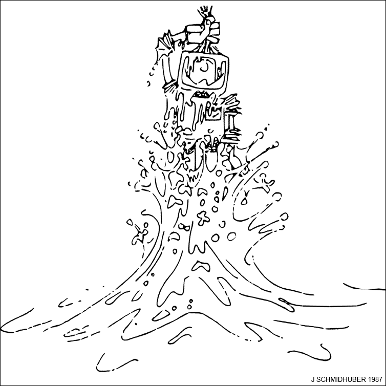
For its cover I drew a robot that bootstraps itself.
1992-: gradient descent-based neural metalearning. 1994-: Meta-Reinforcement Learning with self-modifying policies. 1997: Meta-RL plus artificial curiosity and intrinsic motivation.
2002-: asymptotically optimal metalearning for curriculum learning. 2003-: mathematically optimal Gödel Machine. 2020: new stuff!
.